Plots for Continuous Distributions
Importing
To use the continuous plots, you must import the plots module. Plot_continuous and Plot_norm are the only functions that don’t require you to import the plots module.
In [1]: from prob140.plots import *
Quick Reference
The normal syntax for plotting a distribution is Plot_distribution(x_limits, parameters, optional_arguments)
Click the links below to see detailed information for plotting any distribution. Note that we won’t use most of these for Prob140
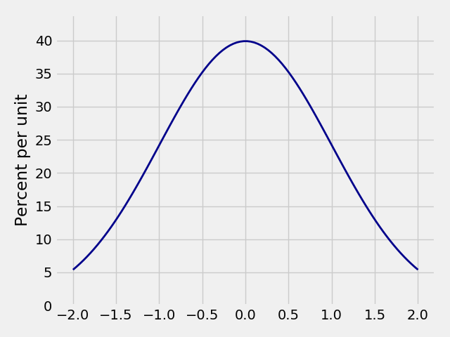
Plot_norm(x_limits, mu, sigma, **kwargs) |
Plots a gaussian distribution. |
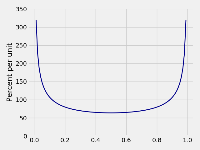
Plot_arcsine(x_limits, **kwargs) |
Plots an arcsine distribution. |
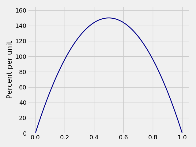
Plot_beta(x_limits, a, b, **kwargs) |
Plots a beta distribution. |
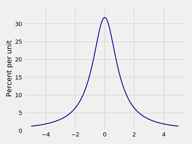
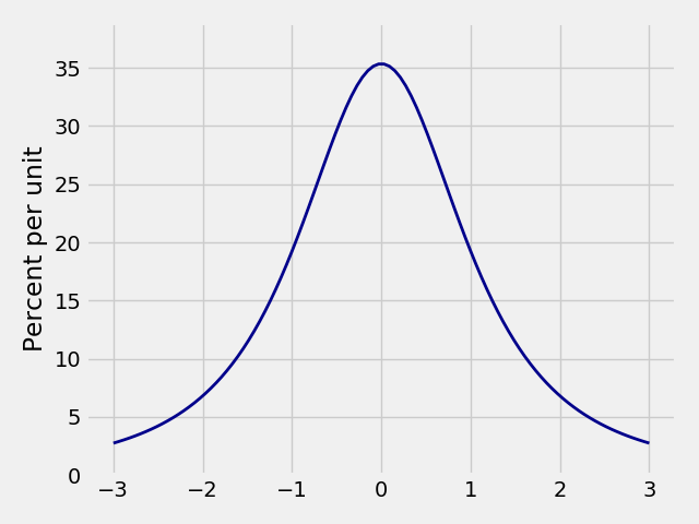
Plot_cauchy(x_limits[, loc, scale]) |
Plots a cauchy distribution. |
Plot_chi2(x_limits, df, **kwargs) |
Plots a chi-squared distribution. |
Plot_erlang(x_limits, r, lamb, **kwargs) |
Plots an erlang distribution. |
Plot_expon(x_limits, lamb, **kwargs) |
Plots an exponential distribution |
Plot_f(x_limits, dfn, dfd, **kwargs) |
Plots an F distribution. |
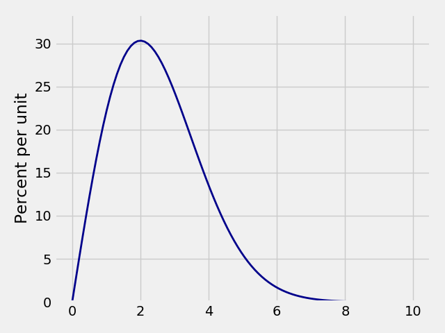
Plot_gamma(x_limits, r, lamb, **kwargs) |
Plots a gamma distribution. |
Plot_lognorm(x_limits, mu, sigma, **kwargs) |
Plots a log-normal distribution. |
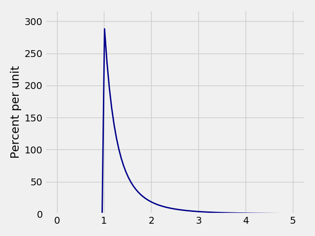
Plot_pareto(x_limits, alpha, **kwargs) |
Plots an alpha distribution. |
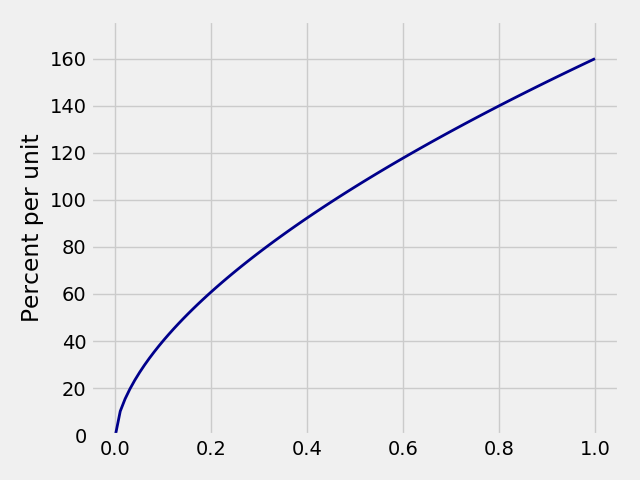
Plot_powerlaw(x_limits, a, **kwargs) |
Plots a powerlaw distribution. |
Plot_rayleigh(x_limits, sigma, **kwargs) |
Plots a rayleigh distribution. |
Plot_t(x_limits, df, **kwargs) |
Plots a t distribution. |
Plot_triang(x_limits, a, b, c, **kwargs) |
Plots a triangular distribution. |
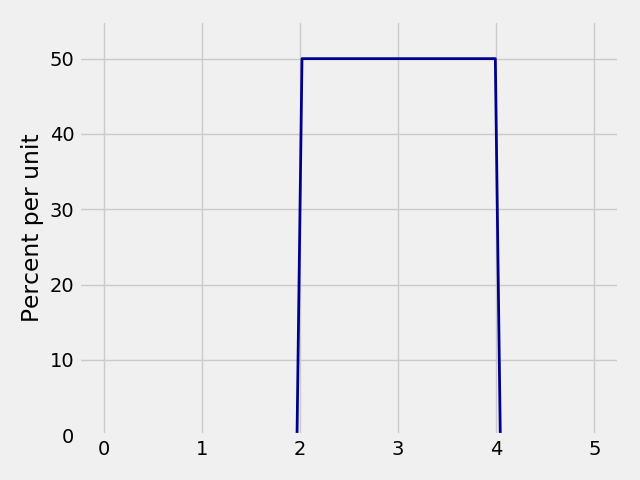
Plot_uniform(x_limits, a, b, **kwargs) |
Plots a uniform distribution. |
Plot_continuous(x_limits, func, *args, **kwargs) |
Plots a continuous distribution |
Plotting events
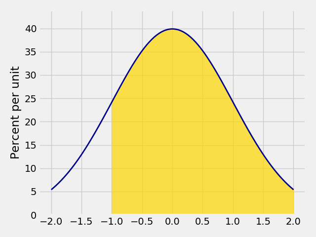
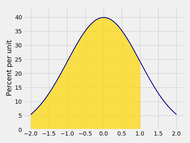
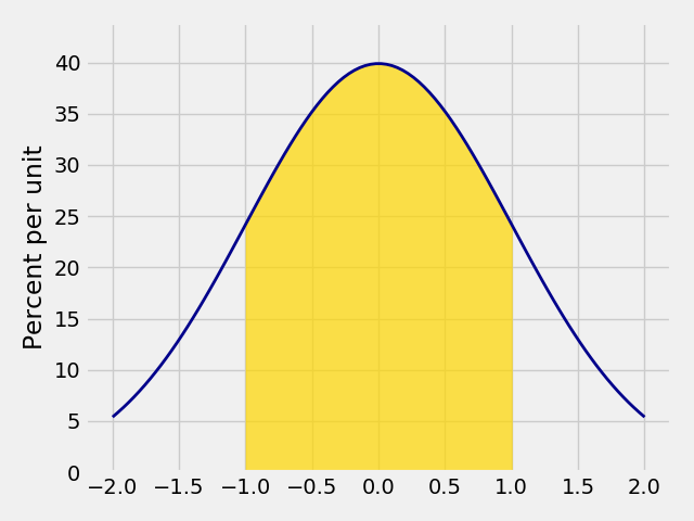
The optional parameters left_end= and right_end= define the left and right side to be shaded. These optional parameters should work for all the continuous distribution plots
In [2]: Plot_norm(x_limits=(-2, 2), mu=0, sigma=1, left_end=-1)
In [3]: Plot_norm(x_limits=(-2, 2), mu=0, sigma=1, right_end=1)
In [4]: Plot_norm(x_limits=(-2, 2), mu=0, sigma=1, left_end=-1, right_end=1)
We can also set the parameter tails=True to invert the direction to be shaded.
In [5]: Plot_norm(x_limits=(-2, 2), mu=0, sigma=1, left_end=-1, right_end=1, tails=True)

CDF
For all the plot functions except Plot_continuous, you can pass the parameter cdf=True to plot the cumulative distribution function instead of the probability density function. This also works with left_end/right_end
In [6]: Plot_norm(x_limits=(-2, 2), mu=0, sigma=1, cdf=True)


