Long Run Behavior
Long Run Behavior
By conditioning on $X_n$, we have seen that for any state $j$,
$$ P(X_{n+1} = j) = P_{n+1}(j) = \sum_{i \in S} P_n(i)P(i, j) $$In principle, this allows us to calculate the distributions $P_n$ sequentially, starting with the inital distribution and transition matrix. That's what the distribution method does.
The input for distribution is a numerical transition matrix. Symbolic calculations, on the other hand, can quickly get intractable, and indeed, so can numerical calculations when the state space and run time of the chain are both large.
To see why, let's try to get a sense of what is involved. Suppose $n \ge 1$ and let $i$ and $j$ be any two states. The one-step transition probability $P_1(i, j)$ is just $P(i, j)$ which can be read off the transition matrix. Next, by conditioning on the first move,
$$ P_2(i, j) = \sum_{k \in S} P_1(i, k)P(k, j) = \sum_{k \in S} P(i, k)P(k, j) $$If you have taken some linear algebra you will recognize this as an element in the product of the transition matrix with itself. Indeed, if you denote the 2-step transition matrix by $\mathbb{P}_2$, then
$$ \mathbb{P}_2 = \mathbb{P}^2 $$By induction, the $n$-step transition matrix is $$ \mathbb{P}_n = \mathbb{P}^n $$
The $n$-step transition matrix is the $n$th power of the one-step transition matrix.
Raising a large matrix to a large power is a formidable operation. Yet it is important to understand how the chain behaves in the long run. Fortunately, a marvelous theorem comes to the rescue.
Convergence to Stationarity
Every irreducible and aperiodic Markov Chain with a finite state space exhibits astonishing regularity after it has run for a while.
For such a chain, for all states $i$ and $j$,
$$ P_n(i, j) \to \pi(j) ~~~ \text{as } n \to \infty $$That is, the $n$-step transition probability from $i$ to $j$ converges to a limit that does not depend on $i$. Moreover,
$\pi(j) > 0$ for all states $j$, and
$\sum_{j \in S} \pi(j) = 1$
That is, as $n \to \infty$, the limit $\pi$ of the distributions $P_n$ is a probability distribution in which all terms are positive. It is called the stationary or invariant or steady state distribution of the chain.
The proof of this theorem is beyond the scope of this course. In fact the result is true in greater generality, for some classes of Markov Chains on infinitely many states. In Prob140 we will assume that it is true for irreducible aperiodic finite state chains, and then see what it implies.
First, let's recall that we have seen this behavior in examples. Here is the transition diagram for a lazy reflecting random walk on five states.
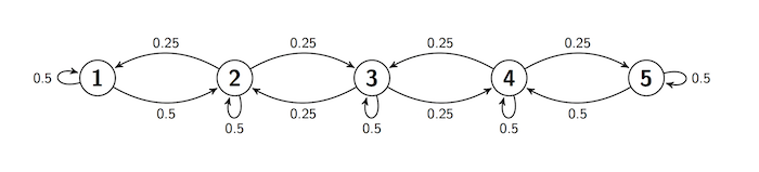
Here is the same information in a transition matrix.
def ref_walk_probs(i, j):
    if i-j == 0:
        return 0.5
    elif 2 <= i <= 4:
        if abs(i-j) == 1:
            return 0.25
        else:
            return 0
    elif i == 1:
        if j == 2:
            return 0.5
        else:
            return 0
    elif i == 5:
        if j == 4:
            return 0.5
        else:
            return 0

trans_tbl = Table().states(s).transition_function(ref_walk_probs)
refl_walk = trans_tbl.toMarkovChain()
refl_walk
Let's start the chain out with an arbitrary initial distribution.
s = np.arange(1, 6)
init_probs = [0.1, 0.2, 0.3, 0.25, 0.15]
initial = Table().states(s).probability(init_probs)
initial
Here is $P_3$, the distribution of $X_3$. This is what we are calling the "distribution at time 3".
refl_walk.distribution(initial, 3)
Here is the distribution at time 100:
refl_walk.distribution(initial, 100)
And here it is at time 200:
refl_walk.distribution(initial, 200)
As the theorem predicts, the distribution at time $n$ has a limit as $n$ gets large. The limit is a probability distribution whose elements are all positive.
Forgetting Where it Came From
Let's start the chain out with a different initial distribution; one that puts all its mass at state 3. The limit distribution is still the same.
initial2 = Table().states(s).probability([0, 0, 1, 0, 0])
refl_walk.distribution(initial2, 100)
As the theorem says, $\lim_n P_n(i, j)$ is $\pi(j)$, which depends on the end state $j$ but not on the start state $i$. In the long run, a Markov Chain forgets where it started.
Balance Equations
The distribution method is a way to identify the stationary distribuion $\pi$ if you have a numerical transition matrix and a computer equipped with the prob140 Python library. But there is a more general way of finding $\pi$.
Let $n \ge 0$ and let $i$ and $j$ be two states. Then
$$ P_{n+1}(i, j) = \sum_{k \in S} P_n(i, k)P(k, j) $$Therefore
\begin{align*} \lim_{n \to \infty} P_{n+1}(i, j) &= \lim_{n \to \infty} \sum_{k \in S} P_n(i, k)P(k, j) \\ \\ &= \sum_{k \in S} \big{(} \lim_{n \to \infty} P_n(i, k) \big{)} P(k, j) \end{align*}We can exchange the limit and the sum because $S$ is finite. Now apply the theorem on convergence to stationarity:
$$ \pi(j) = \sum_{k \in S} \pi(k)P(k, j) $$These are called the balance equations.
In matrix notation, if you think of $\pi$ as a row vector, these equations become
$$ \pi = \pi \mathbb{P} ~~~~~ \text{or, equivalently,} ~~~~~ \pi\mathbb{P} = \pi $$Let's see how this works out for our lazy reflecting random walk. Here is its transition matrix:
refl_walk
According to the balance equations,
$$ \pi(1) = \sum_{k=1}^s \pi(k)P(k, 1) $$That is, we're multiplying $\pi$ by the 1 column of $\mathbb{P}$ and adding. So
Follow the same process to get all five balance equations:
\begin{align*} \pi(1) &= 0.5\pi(1) + 0.25\pi(2) \\ \pi(2) &= 0.5\pi(1) + 0.5\pi(2) + 0.25\pi(3) \\ \pi(3) &= 0.25\pi(2) + 0.5\pi(3) + 0.25\pi(4) \\ \pi(4) &= 0.25\pi(3) + 0.5\pi(4) + 0.5\pi(5) \\ \pi(5) &= 0.25\pi(4) + 0.5\pi(5) \end{align*}Some observations make the system easy to solve.
- By rearranging the first equation, we get $\pi(2) = 2\pi(1)$.
- By symmetry, $\pi(1) = \pi(5)$ and $\pi(2) = \pi (4)$.
- Because $\pi(2) = \pi(4)$, the equation for $\pi(3)$ shows that $\pi(3) = \pi(2) = \pi(4)$.
So the distribution $\pi$) is $$ \big{(} \pi(1), 2\pi(1), 2\pi(1), 2\pi(1), \pi(1) \big{)} $$
As $\pi$ is a probability distribution, it sums to 1. As its total is $8\pi(1)$, we have
$$ \pi = \big{(} \frac{1}{8}, \frac{2}{8}, \frac{2}{8}, \frac{2}{8}, \frac{1}{8} \big{)} $$This agrees with what we got by using distribution for $n=100$. In fact we could just have used the method steady_state to get $\pi$:
refl_walk.steady_state()
The steady state isn't an element of the state space $S$ – it's the condition of the chain after it has been run for a long time. Let's examine this further.
Balance and Steady State
To see what is being "balanced" in these equations, imagine a large number of independent replications of this chain. For example, imagine a large number of particles that are moving among the states 1 through 5 according to the transition probabilities of the lazy reflectin walk, and suppose all the particles are moving at instants 1, 2, 3, $\ldots$ independently of each other.
Then at any instant and for any state $j$, there is some proportion of particles that is leaving $j$, and another proportion that is entering $j$. The balance equations say that those two proportions are equal.
Let's check this by looking at the equations again: for any state $j$,
$$ \pi(j) = \sum_{k \in S} \pi(k)P(k, j) $$For every $k \in S$ (including $k=j$), think of $\pi(k)$ as the proportion of particles leaving state $k$ after the chain has been run a long time. Then the left hand side is the proportion leaving $j$. The generic term in the sum on the right is the proportion that left $k$ at the previous instant and are moving to $j$. Those are the particles entering $j$. When the two sides are equal, the chain is balanced.
The theorem on convergence to stationarity says that the chain approaches balance as $n$ gets large. If it actually achieves balance, that is, if $P_n = \pi$ for some $n$, then it stays balanced. The reason:
$$ P_{n+1}(j) = \sum_{i \in S} P_n(i)P(i, j) = \sum_{i \in S} \pi(i)P(i, j) = \pi(j) $$by the balance equations.
In particular, if you start the chain with its stationary distribution $\pi$, then the distribution of $X_n$ is $\pi$ for every $n$.
Uniqueness
It's not very hard to show that if a probability distribution solves the balance equations, then it has to be $\pi$, the limit of the marginal distributions of $X_n$. We won't do the proof; it essentially repeats the steps we took to derive the balance equations. You should just be aware that an irreducible, aperiodic, finite state Markov Chain has exactly one stationary distribution.
This is particularly helpful if you happen to guess a solution to the balance equations. If the solution that you have guessed is a probability distribution, you have found the stationary distribution of the chain.
Expected Long Run Proportion of Time
Let $j$ be a state, and let $I_m(j)$ be the indicator of the event $\{X_m = j\}$. The proportion of time the chain spends at $j$, from time 1 through time $n$, is
$$ \frac{1}{n} \sum_{m=1}^n I_m(j) $$Therefore, the expected proportion of time the chain spends at $j$, given that it started at $i$, is
$$ \frac{1}{n} \sum_{m=1}^n E(I_m(j) \mid X_0 = i) = \frac{1}{n} \sum_{m=1}^n P(X_m = j \mid X_0 = i) = \frac{1}{n} \sum_{m=1}^n P_m(i, j) $$Now recall a property of convergent sequences of real numbers: If $x_n \to x$ as $n \to \infty$, then the sequence of averages also converges to $x$: $$ \frac{1}{n} \sum_{m=1}^n x_m \to x ~~~ \text{as } n \to \infty $$
Take $x_n = P_n(i, j)$. Then by the theorem on convergence to stationarity,
$$ P_n(i, j) \to \pi(j) ~~~ \text{as } n \to \infty $$and hence the averages also converge: $$ \frac{1}{n} \sum_{m=1}^n P_m(i, j) \to \pi(j) ~~~ \text{as } n \to \infty $$
Thus the long run expected proportion of time the chain spends in state $j$ is $\pi(j)$, where $\pi$ is the stationary distribution of the chain.
For example, the lazy reflecting random walk of this section is expected to spend about 12.5% of its time at state 1, 25% of its time at each of states 2, 3, and 4, and the remaining 12.5% of its time at state 5.