Poissonization
Poissonization
A binomial $(n, p)$ random variable has a finite number of values: it can only be between 0 and $n$. But now that we are studying the behavior of binomial probabilities as $n$ gets large, it is time to move from finite outcome spaces to spaces that are infinite.
Our first example of a probability distribution on infinitely many values is motivated by the approximation we developed for binomial $(n, p)$ probabilities when $n$ is large and $p$ is small. Under these conditions we saw that the chance of $k$ successes in $n$ i.i.d. Bernoulli $(p)$ trials is roughly
$$ P(k) \approx e^{-\mu} \frac{\mu^k}{k!}, ~~ k = 0, 1, 2, \ldots, n $$for $\mu = np$.
The terms in the approximation are proportional to terms in the series expansion of $e^\mu$, but that expansion is infinite. We don't have to stop at $n$, so we won't.
But a little care is required before we go further. First, we must state the additivity axiom of probability theory in terms of countably many outcomes:
$$ P(\bigcup_{i=1}^\infty A_i) = \sum_{i=1}^\infty P(A_i) $$This is called the countable additivity axiom, in contrast to the finite additivity axiom we have thus far assumed.
In this course, we will not go into the technical aspects of countable additivity and the existence of probability functions that satisfy the axioms on the spaces that interest us. But those technical aspects do have to be studied before you can develop a deeper understanding of probability theory. If you want to do that, a good start is to take Real Analysis and then Measure Theory.
But while in Prob140, you don't have to worry about it. Just assume that all the distributions that we describe do in fact satisfy the axioms. Here is our first infinite valued distribution.
Poisson Distribution
A random variable $X$ has the Poisson distribution with parameter $\mu > 0$ if
$$ P(X = k) = e^{-\mu} \frac{\mu^k}{k!}, ~~ k = 0, 1, 2, \ldots $$The terms are proportional to the terms in the infinte series expansion of $e^{\mu}$. These terms of $\mu^k/k!$ for $k \ge 0$ determine the shape of the distribution.
The constant of proportionality is $e^{-\mu}$. It doesn't affect the shape; it just ensures that the probabilities add up to 1.
$$ \sum_{k=0}^\infty P(X = k) = \sum_{k=0}^\infty e^{-\mu} \frac{\mu^k}{k!} = e^{-\mu} \sum_{k=0}^\infty \frac{\mu^k}{k!} = e^{-\mu} \cdot e^{\mu} = 1 $$The Poisson is a distribution in its own right. It does not have to arise as a limit of binomials, though it is often helpful to think of it that way.
The Mode
To understand the parameter $\mu$ of the Poisson distribution, a first step is to notice that mode of the distribution is just around $\mu$. Here is an example where $\mu = 3.74$. No computing system can calculate infinitely many probabilities, so we have just calculated the Poisson probabilities till the sum is close enough to 1 that the prob140 library considers it a Distribution object.
mu = 3.74
k = range(20)
poi_probs_374 = stats.poisson.pmf(k, mu)
poi_dist_374 = Table().values(k).probability(poi_probs_374)
Plot(poi_dist_374)
plt.title('Poisson (3.74)');
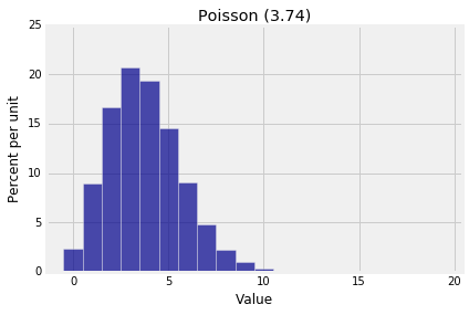
The mode is 3. To find a formula for the mode, follow the process we used for the binomial: calculate the consecutive odds ratios, notice that they are decreasing, and see where they cross 1. This is left to you as an exercise. Your calculations should conclude the following:
Mode of the Poisson
The mode of the Poisson distribution is the integer part of $\mu$; that is, the most likely value is $\mu$ rounded down to an integer. If $\mu$ is an integer, both $\mu$ and $\mu - 1$ are modes.
mu = 4
k = range(20)
poi_probs_4 = stats.poisson.pmf(k, mu)
poi_dist_4 = Table().values(k).probability(poi_probs_4)
Plot(poi_dist_4)
plt.ylim(0, 25)
plt.title('Poisson (4)');
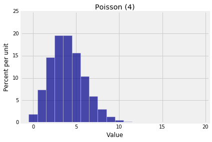
In later chapters we will learn a lot more about the parameter $\mu$ of the Poisson distribution. For now, just keep in mind that the most likely value is essentially $\mu$.
The Cumulative Distribution Function (c.d.f.)
Very often, we need probabilities of the form $P(X > x)$ or $P(X \le x)$. For example, if $X$ has the Poisson $(4)$ distribution, here is the event $\{ X \le 5 \}$.
Plot(poi_dist_4, event=range(6))
plt.ylim(0, 25)
plt.title('Poisson (4)');
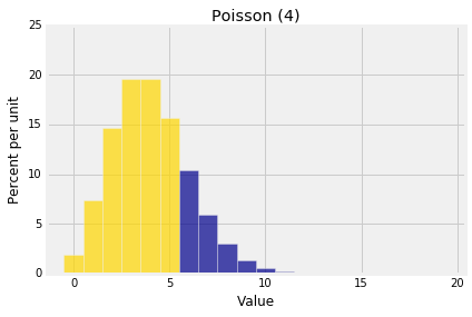
The cumulative distribution function or c.d.f. of any random variable is a function that calculates this "area to the left" of any point. If you denote the c.d.f. by $F$, then $$ F(x) = P(X \le x) $$ for any x.
We will get to know this function better later in the term. For now, note that stats lets you calculate it directly without having to use pmf and then summing. The function is called stats.distribution_name.cdf where distribution_name could be binom or poisson or any other distribution name that stats recognizes. The first argument is $x$, followed by the arguments of the distribution. In the case of the Poisson, there is just one argument $\mu$.
For $X$ a Poisson $(4)$ random variable, the gold area above is $P(X \le 5)$ which is about 78.5%.
stats.poisson.cdf(5, 4)