Binomial Distribution
The Binomial Distribution
Let $X_1, X_2, \ldots , X_n$ be i.i.d. Bernoulli $(p)$ random variables and let $S_n = X_1 + X_2 \ldots + X_n$. That's a formal way of saying:
- Suppose you have a fixed number $n$ of success/failure trials; and
- the trials are independent; and
- on each trial, the probability of success is $p$.
- Let $S_n$ be the total number of successes.
The first goal of this section is to find the distribution of $S_n$.
In the example that we fixed our minds on earlier, we were counting the number of sixes in 7 rolls of a die. The 7 rolls are independent of each other, the chance of "success" (getting a six) is $1/6$ on each trial, and $S_7$ is the number of sixes.
The first step in finding the distribution of any random variable is to identify the possible values of the variable. In $n$ trials, the smallest number of successes you can have is 0 and the largest is $n$. So the set of possible values of $S_n$ is $\{0, 1, 2, \ldots , n\}$.
Thus the number of sixes in 7 rolls can be any integer in the 0 through 7 range. For $k = 3$, let's find $P(S_7 = 3)$.
Partition the $\{S_7 = 3\}$ into the different ways it can happen. One way can be denoted SSSFFFF, where S denotes "success" (or "six"), and F denotes failure. Another is SFFSSFF. And so on.
Now notice that
$$ P(\text{SSSFFFF}) = \big{(}\frac{1}{6}\big{)}^3 \big{(}\frac{5}{6}\big{)}^4 = P(\text{SFFSSFF}) $$by independence. Indeed, any sequence of three S's and four F's has the same probability. So by the addition rule,
\begin{align*} P(S_7 = 3) &= \text{(number of sequences of three S and four F)} \cdot \big{(}\frac{1}{6}\big{)}^3 \big{(}\frac{5}{6}\big{)}^4 \\ \\ &= \binom{7}{3} \big{(}\frac{1}{6}\big{)}^3 \big{(}\frac{5}{6}\big{)}^4 \end{align*}because $\binom{7}{3}$ counts the number of ways you can choose 3 places out of 7 in which to put the symbol S; the remaining 4 get filled with F.
An analogous argument leads us to one of the most important distributions in probability theory.
The Binomial $(n, p)$ Distribution
Let $S_n$ be the number of successes in $n$ independent Bernoulli $(p)$ trials. Then $S_n$ has the binomial distribution with parameters $n$ and $p$, defined by
$$ P(S_n = k) = \binom{n}{k} p^k (1-p)^{n-k}, ~~~ k = 0, 1, \ldots, n $$Parameters of a distribution are constants associated with it. For example, the Bernoulli $(p)$ distribution has parameter $p$. The binomial distribution defined above has parameters $n$ and $p$ and is called the binomial $(n, p)$ distribution.
Before we get going on calculations with this distribution, let's make a few observations.
- The functional form of the probabilities is symmetric in successes in failures, because
That's "number of trials, factorial; divided by number of successes factorial times number of failures factorial; times the probability of success to the power number of successes; times the probability of failure to the power number of failures.
- The formula makes sense for the edge cases $k=0$ and $k=n$. We can calculate $P(S_n = 0)$ without any of the machinery developed above. It's the chance of no successes, which is the chance of all failures, which is $(1-p)^n$. Our formula says $$ P(S_n = 0) = \frac{n!}{0!(n-0)!} p^0 (1-p)^{n-0} = (1-p)^n $$ after all the dust clears in the formula; the first two factors are both 1. You can check that $P(S_n = 0) = p^n$, the chance that all the trials are successes.
Remember that $0! = 1$ by definition. In part, it is defined that way to make the formula for $\binom{n}{k}$ work out correctly when $k=0$. There is also another reason which you will see later in the course.
- The probabilities in the distribution sum to 1. To see this, recall that for any two numbers $a$ and $b$,
by the binomial expansion of $(a+b)^n$. The numbers $\binom{n}{k}$ are the elements of Pascal's triangle, as you will have seen in a math class.
Now plug in $a = p$ and $b = 1-p$ and notice that the terms in the sum are exactly the binomial probabilities we defined above. So the sum of the probabilities is
$$ \sum_{k=0}^n \binom{n}{k} p^k (1-p)^{n-k} ~ = ~ \big{(} p + (1-p) \big{)}^n ~ = ~ 1^n ~ = ~ 1 $$Binomial Probabilities in Python
The stats submodule of the scipy module does numerous calculations in probability and statistics. We will be importing it at the start of every notebook from now on.
from scipy import stats
The function stats.binom.pmf takes three arguments: $k$, $n$, and $p$, in that order. It returns the numerical value of $P(S_n = k)$ For short, we will say that the function returns the binomial $(n, p)$ probability of $k$.
The acronym "pmf" stands for "probability mass function" which as we have noted earlier is sometimes used as another name for the distribution of a variable that has finitely many values.
The chance of 3 sixes in 7 rolls of a die is thus $\binom{7}{3}(1/6)^3(5/6)^4$ by the binomial formula, which works out to about 8%:
stats.binom.pmf(3, 7, 1/6)
You can also specify an array or list of values of $k$, and stats.binom.pmf will return an array consisting of all their probabilities.
stats.binom.pmf([2, 3, 4], 7, 1/6)
Thus to find $P(2 \le S_7 \le 4)$, you can use
sum(stats.binom.pmf([2, 3, 4], 7, 1/6))
Binomial Histograms
To visualize binomial distributions we will use the prob140 method Plot as we have done earlier, after first using stats.binom.pmf to calculate the binomial probabilities. The cell below plots the distribution of $S_7$ above. Notice how we start by specify all the possible values of $S_7$ in the array k.
n = 7
p = 1/6
k = np.arange(n+1)
binom_7_16 = stats.binom.pmf(k, n, p)
binom_7_16_dist = Table().values(k).probability(binom_7_16)
Plot(binom_7_16_dist)
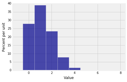
Not surprisingly, the graph shows that in 7 rolls of a die you are most likely to get around 1 six.
This distribution is not symmetric, as you would expect. But something interesting happens to the distribution of the number of sixes when you increase the number of rolls.
n = 600
p = 1/6
k = np.arange(n+1)
binom_600_16 = stats.binom.pmf(k, n, p)
binom_600_16_dist = Table().values(k).probability(binom_600_16)
Plot(binom_600_16_dist)
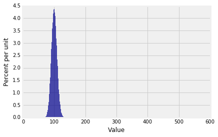
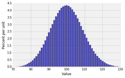
Notice that while the the possible values of the number of sixes range from 0 to 600, the probable values are in a much smaller range. The plt.xlim function allows us to zoom in on the probable values. The semicolon is just to prevent Python giving us a message that clutters up the graph. The edges=True option forces Plot to draw lines separating the bars; by default, it stops doing that if the number of bars is large.
Plot(binom_600_16_dist, edges=True)
plt.xlim(70, 130);
Does the binomial $(n, p)$ distribution always look bell shaped if $n$ is large? It does not.
Something quite different happens if your random variable is the number of successes in 600 trials that have probability 1/600 of success on each trial. Then the distribution of the number of successes is binomial $(600, 1/600)$, which looks like this:
n = 600
p = 1/600
k = np.arange(n+1)
binom_600_1600 = stats.binom.pmf(k, n, p)
binom_600_1600_dist = Table().values(k).probability(binom_600_1600)
Plot(binom_600_1600_dist)
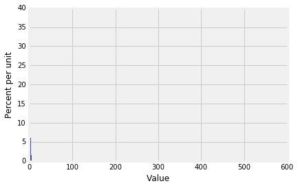
We really can't see that at all! Let's zoom in.
Plot(binom_600_1600_dist, edges=True)
plt.xlim(0, 10);
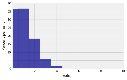
That's annoying. Half of the bar over 0 is cut off because the bar is centered at 0. So instead:
Plot(binom_600_1600_dist, edges=True)
plt.xlim(-1, 10);
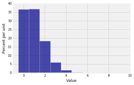
Now you can see that in 600 independent trials with probability 1/600 of success on each trial, you are most likely to get no successes or 1 success. There is some chance that you get 2 through 4 successes, but the chance of any number of successes greater than 4 is barely visible on this scale.
Clearly, the shape of the histogram is determined by both $n$ and $p$. We will study the shape carefully in an upcoming section. But first, let's do some numerical examples of using the binomial distribution.