Updating Probabilities
Updating Probabilities
Data changes minds. We might start out with a set of assumptions about how the world works, but as we gather more data, we may have to update our opinions.
Probabilities too can be updated as information comes in. As you saw in Data 8, Bayes' Rule is one way to update probabilities. Let's recall the rule in the context of an example, and then we will state it in greater generality.
Example: Using Bayes' Rule
In a population there is a rare disease: only 0.4% of the people have it. There is a laboratory test for the disease that has a 99% chance of returning a positive result when run on a person that has the disease. When run on someone who doesn't have the disease, it has a 99.5% chance of returning a negative result. So overall, it's a pretty good test.
One person is picked at random from this population. Given that the person tests positive, what is the chance that the person has the disease?
Here is the tree diagram we drew in Data 8, to summarize the information in the problem.
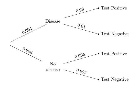
To solve the problem, we will use the division rule as we did in Data 8. In this kind of application, where we are finding probabilities for an earlier phase of an experiement given the result of a later phase, the division rule is called Bayes' Rule.
Let $D$ be the event that the patient has the disease, and, with some abuse of math notation, let $+$ be the event that the patient tests positive. Then what we're looking for is $P(D \mid +)$. By the division rule,
$$ P(D \mid + ) = \frac{P(D \text{ and } +)}{P(+)} = \frac{0.004 \cdot 0.99}{0.004 \cdot 0.99 + 0.996 \cdot 0.005} = 44.3\% $$(.004*.99)/(0.004*.99 + 0.996*.005)
Bayes' Rule
In general, if the entire outcome space can be partitioned into events $A_1, A_2 \ldots , A_n$, and $B$ is an event of positive probability, then for each $i$,
\begin{align*} P(A_i \mid B) &= \frac{P(A_iB)}{P(B)} ~~~~ \text{(division rule)} \\ \\ &= \frac{P(A_iB)}{\sum_{j=1}^n P(A_j B)} ~~~~ \text{(the }A_j\text{'s partition the whole space)} \\ \\ &= \frac{P(A_i)P(B \mid A_i)}{\sum_{j=1}^n P(A_j)P(B \mid A_j)} ~~~~ \text{(multiplication rule)} \end{align*}This calculation, called Bayes' Rule, is an application of the division rule in a setting where the events $A_1, A_2, \ldots , A_n$ can be thought of as the results of an "earlier" stage of an experiment and $B$ the result of a "later" stage. The calculation allows us to find "backwards in time" conditional chances of an earlier event given a later one, by writing the chance in terms of the "forwards in time" conditional chances of the later event given the earlier ones.
The Effect of the Prior
Now let's take a look at the numerical value of the answer we got in our example. It's a bit disconcerting: it says that even though the person has tested positive, there is less than 50% chance they have the disease: the disease is so rare that the proportion of people who have the disease and test positive is actually a bit smaller than the people who don't have the disease and get a bad test result.
This is not a fault of the test. It's due to our premise, that the person "is picked at random from the population." That's not what happens when people go to get tested. Usually they go because they or their doctors think they should. And in that case they are no longer "randomly picked" members of the population.
If a person thinks they might have the disease, then their subjective probability of having the disease should be larger than the probability for a random member of the population. Let's take the following steps to see how much difference the prior makes.
- We will change the "prior probability" of disease from 0.004 to other values; the prior probability of "no disease" will change correspondingly.
- We will leave the test accuracy unchanged.
- We will observe the changes in the "posterior probability" of disease given that the person tested positive, for different values of the prior.
prior = make_array(0.004, 0.01, 0.05, 0.1, 0.5)
Table().with_columns(
   'Prior P(D)', prior,
    'Posterior P(D|+)', (prior*0.99)/(prior*0.99 + (1-prior)*0.005)
)
You can see that the posterior chance that the person has the disease, given that they tested positive, depends heavily on the prior. For example, if the person thinks they even have a 10% chance of the disease, then, given that they test positive, their probability of having the disease gets updated to over 95%.
Prior, Likelihood, and Posterior
Another way to visualize this is by defining a Bernoulli random variable $X$ that is 1 if the person has the disease and 0 otherwise. We say that "$X$ is the indicator of the person having the disease."
Suppose the person starts out with a 10% prior probability that they have the disease. Then $X$ is Bernoulli $(0.1)$.
How you update this distribution based on test results depends not only on the prior but also on the likelihood that the person tests positive given that they have or don't have the disease. This likelihood derives from the accuracy of the test, which is 99% if the person has the disease and 99.5% if they don't.
To see how all these different aspects fit together, define a new Bernoulli random variable $T$ that is 1 if the test result is positive and 0 if the test result is negative. So $T$ is the indicator of the person testing positive. The joint distribution of $X$ and $T$ is displayed in the following table.
x = make_array(0, 1)
t = make_array(0, 1)
def jt(t, x):
    if x == 1:
        if t == 1:
            return 0.1*0.99
        if t == 0:
            return 0.1*0.01
    if x == 0:
        if t == 1:
            return 0.9*0.005
        if t == 0:
            return 0.9*0.995

dist_xt_tbl = Table().values('T', t, 'X', x).probability_function(jt)
dist_xt = dist_xt_tbl.toJoint()
dist_xt
The entry in each $(x, t)$ cell is $P(X=x)P(T=t \mid X=x)$, that is, the "prior times the likelihood".
Each entry in the T=1 column of the joint distribution table has the form prior times likelihood, and the conditional distribution of $X$ given $T=1$ is obtained by dividing those products by the same quantity $P(T=1)$. This conditional distribution, called the posterior distribution of $X$ given $T=1$, thus satisfies
dist_xt.conditional_dist('X', 'T')
You can see that the posterior distribution of $X$ given $T=1$ is consistent with the posterior probability $P(D \mid +)$ we calculated in an earlier table in the case $P(D) = 0.1$.