Examples
Here are two examples to illustrate how to find the stationary distribution and how to use it.
A Diffusion Model by Ehrenfest
Paul Ehrenfest proposed a number of models for the diffusion of gas particles, one of which we will study here.
The model says that there are two containers containing a total of N particles. At each instant, a container is selected at random and a particle is selected at random independently of the container. Then the selected particle is placed in the selected container; if it was already in that container, it stays there.
Let Xn be the number of particles in Container 1 at time n. Then X0,X1,… is a Markov chain with transition probabilities given by:
P(i,j)={N−i2Nif j=i+112if j=ii2Nif j=i−10otherwiseThe chain is clearly irreducible. It is aperiodic because P(i,i)>0.
Question. What is the stationary distribution of the chain?
Answer. We have computers. So let’s first find the stationary distribution for N=100 particles, and then see if we can identify it for general N.
N = 100

states = np.arange(N+1)

def transition_probs(i, j):
    if j == i:
        return 1/2
    elif j == i+1:
        return (N-i)/(2*N)
    elif j == i-1:
        return i/(2*N)
    else:
        return 0

ehrenfest = MarkovChain.from_transition_function(states, transition_probs)
Plot(ehrenfest.steady_state(), edges=True)
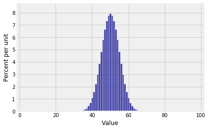
That looks suspiciously like the binomial (100, 1/2) distribution. In fact it is the binomial (100, 1/2) distribution. Since you’ve guessed it, all you have to do is plug it into the balance equations and check that they work out.
The balance equations are:
π(0)=12π(0)+12Nπ(1)π(j)=N−(j−1)2Nπ(j−1)+12π(j)+j+12Nπ(j+1), 1≤j≤N−1π(N)=12Nπ(N−1)+12π(N)You have already guessed the solution by looking at the answer calculated for N=100. But if you want to start from scratch, you’ll have to simplify the balance equations.
To do this, it’s a great idea to write all the elements of π in terms of one of the elements.
Try writing all the elements of π in terms of π(0). You will get:
π(1)=Nπ(0)π(2)=N(N−1)2π0=(N2)π(0)and so on by induction:
π(j)=(Nj)π(0)In other words, the stationary distribution is proportional to the binomial coefficients. So π(0)=1/2N to make all the elements sum to 1, and the distribution is binomial (N,1/2).
Expected Reward
Suppose I run the sticky reflecting random walk from the previous section for a long time. As a reminder, here is its stationary distribution.
stationary = reflecting_walk.steady_state()
stationary
| Value | Probability |
|---|---|
| 1 | 0.125 |
| 2 | 0.25 |
| 3 | 0.25 |
| 4 | 0.25 |
| 5 | 0.125 |
Question 1. Suppose that every time the chain is in state 4, I win 4 dollars; every time it’s in state 5, I win 5 dollars; otherwise I win nothing. What is my expected long run average reward?
Answer 1. In the long run, the chain is in steady state. So I expect that on 62.5% of the moves I will win nothing; on 25% of the moves I will win 4 dollars; and on 12.5% of the moves I will win 5 dollars. My expected long run average reward per move is 1.65 dollars.
0*0.625 + 4*0.25 + 5*.125
1.625
Question 2. Suppose that every time the chain is in state i, I toss i coins and record the number of heads. In the long run, how many heads do I expect to get on average per move?
Answer 2. Each time the chain is in state i, I expect to get i/2 heads. When the chain is in steady state, the expected number of coins I toss at any given move is 3. So, by iterated expectations, the long run average number of heads I expect to get is 1.5.
stationary.ev()/2
1.5000000000000013
If that seems artificial, consider this: Suppose I play the game above, and on every move I tell you the number of heads that I get but I don’t tell you which state the chain is in. I hide the underlying Markov Chain. If you try to recreate the sequence of steps that the Markov Chain took, you are working with a Hidden Markov Model. These are much used in pattern recognition, bioinformatics, and other fields.