Confidence Intervals

Interact

Suppose you have a large i.i.d. sample $X_1, X_2, \ldots, X_n$, and let $\bar{X}_n$ be the sample mean. The CLT implies that with chance about 95%, the sample mean is within 2 SDs of the population mean:

$P\big{(}\bar{X}_n \in (\mu - 2\frac{\sigma}{\sqrt{n}}, ~~~ \mu + 2\frac{\sigma}{\sqrt{n}}) \big{)} ~ \approx ~~ 0.95$

png

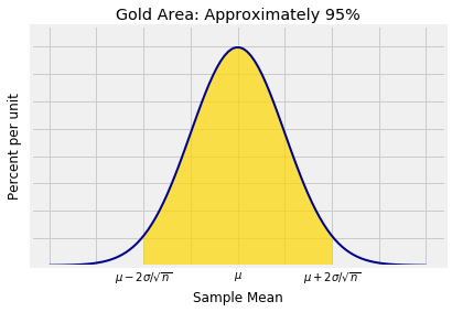
This can be expressed in a different way:

$P\big{(}\vert \bar{X}_n - \mu \vert < 2\frac{\sigma}{\sqrt{n}}\big{)} ~ \approx ~~ 0.95$

Distance is symmetric, so this is the same as saying:

$P\big{(}\mu \in (\bar{X}_n - 2\frac{\sigma}{\sqrt{n}}, ~~~ \bar{X}_n + 2\frac{\sigma}{\sqrt{n}})\big{)} ~ \approx ~~ 0.95$

That is why the interval “sample mean $\pm$ 2 measures of spread” is used as an interval of estimates of $\mu$.

Inverse of the Standard Normal CDF

The interval $\bar{X}_n \pm ~ 2 \sigma/\sqrt{n}$ is called an approximate 95% confidence interval for the parameter $\mu$, the population mean. The interval has a confidence level of 95%. The level determines the use of $z = 2$ as the multiplier of the SD of the sample mean.

You could choose a different confidence level, say 80%. With that choice you would expect the interval to be narrower. To find out exactly how many SDs you have to go on either side of the center to pick up a central area of about 80%, you have to find the corresponding $z$ on the standard normal curve, as shown below.

png

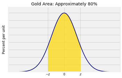
As you know from Data 8 and can see in the figure, the interval runs from the 10th to the 90th percentile of the distribution. So $z$ is the 90th percentile of the standard normal curve, also known as the “90 percent point” of the curve. The scipy method is therefore called ppf and takes a decimal value as its argument.

stats.norm.ppf(.9)

1.2815515655446004

Therefore an approximate 80% confidence interval for the population mean $\mu$ is given by “sample mean $\pm ~ 1.28\sigma/\sqrt{n}$”.

Let’s double check that 2 is a good choice of $z$ for a 95% interval. The $z$ that we need is the 97.5 percent point:

stats.norm.ppf(.975)

1.959963984540054

That’s $z = 1.96$, which we have been calling 2. It’s good enough, but $z = 1.96$ is also commonly used for constructing 95% confidence intervals.

The ppf and cdf functions are inverses of each other.

stats.norm.cdf(1.96), stats.norm.ppf(0.975)

(0.9750021048517795, 1.959963984540054)

In math notation,

$\Phi(z) ~ = ~ p ~~ \iff ~~ \Phi^{-1}(p) = z$

Confidence Interval for Population Mean

Let $\lambda$% be any confidence level. Let $z_\lambda$ be the point such that the interval $(-z_\lambda, ~ z_\lambda)$ contains $\lambda$% of the area under the standard normal curve. In our example above, $\lambda$ was 80 and $z_\lambda$ was 1.28.

Let $p = \lambda/100$ be the value of $\lambda$ converted into a proportion. For example if $\lambda = 80$ then $p = 0.8$. Then

$z_\lambda ~ = ~ \Phi^{-1}(p + 0.5(1-p))$

because all of the area to the left of $z_\lambda$ is the area $p$ between $z_\lambda$ and $-z_\lambda$ plus the tail to the left of $-z_\lambda$.

If $n$ is large,

$p ~ \approx ~ P\big{(}\mu \in (\bar{X}_{n} - z_{\lambda} \frac{\sigma}{\sqrt{n}}, ~~~ \bar{X}_n + z_\lambda \frac{\sigma}{\sqrt{n}})\big{)}$

The random interval $\bar{X}_{n} ~ \pm ~ z_{\lambda} \sigma/\sqrt{n}$ is called an approximate $\lambda$% confidence interval for the population mean $\mu$. There is about a $\lambda$% chance that this random interval contains the parameter $\mu$.

The only difference between confidence intervals of different levels is the choice of $z_\lambda$ which depends on the level $\lambda$. The other two components are the sample mean and its SD.

A Data 8 Example Revisited

Let’s return to an example very familiar from Data 8: a random sample of 1,174 pairs of mothers and their newborns.

baby = Table.read_table('baby.csv')

baby

Birth Weight	Gestational Days	Maternal Age	Maternal Height	Maternal Pregnancy Weight	Maternal Smoker
120	284	27	62	100	False
113	282	33	64	135	False
128	279	28	64	115	True
108	282	23	67	125	True
136	286	25	62	93	False
138	244	33	62	178	False
132	245	23	65	140	False
120	289	25	62	125	False
143	299	30	66	136	True
140	351	27	68	120	False

... (1164 rows omitted)

The third column consists of the ages of the mothers. Let’s construct an approximate 95% confidence interval for the mean age of mothers in the population. We did this in Data 8 using the bootstrap, so we will be able to compare results.

We can apply the methods of this section because our data come from a large random sample.

ages = baby.column('Maternal Age')

samp_mean = np.mean(ages)
samp_mean

27.228279386712096

n = baby.num_rows
n

The observed value of $\bar{X}_n$ in the sample is 27.23 years. We know that $n = 1174$, so all we need is the population SD $\sigma$ and then we can complete our calculation.

But of course we don’t know the population SD $\sigma$. We only have a sample.

As data scientists, we are used to lifting ourselves by our own bootstraps. Notice that the SD of the sample mean is $\sigma/\sqrt{n}$. If we estimate $\sigma$ by the SD of the data, there will be some error in the estimate but the error will be divided by $\sqrt{n}$ and therefore won’t have much effect.

That means we can use “sample SD divided by $\sqrt{n}$” as an estimate of $\sigma/\sqrt{n}$.

The sample SD, our estimate of $\sigma$, is about 5.82 years.

sigma_estimate = np.std(ages)
sigma_estimate

5.815360404190897

An approximate 95% confidence interval for the mean birth weight of babies in the population is $(26.89, 27.57)$ years.

sd_sample_mean = sigma_estimate/(n ** 0.5)

ci_95_pop_mean = samp_mean + 1.96 * make_array(-1, 1) * sd_sample_mean
ci_95_pop_mean

array([26.89562086, 27.56093791])

No bootstrapping required!

Now let’s compare our interval to the interval we got in Data 8 by using the bootstrap percentile method. Here is the function bootstrap_mean from Data 8.

def bootstrap_mean(original_sample, label, replications):
    
    """Displays approximate 95% confidence interval for population mean.
    original_sample: table containing the original sample
    label: label of column containing the variable
    replications: number of bootstrap samples
    """
    just_one_column = original_sample.select(label)
    n = just_one_column.num_rows
    
    means = make_array()
    for i in np.arange(replications):
        bootstrap_sample = just_one_column.sample()
        resampled_mean = np.mean(bootstrap_sample.column(0))
        means = np.append(means, resampled_mean)
        
    left = percentile(2.5, means)
    right = percentile(97.5, means)
    
    resampled_means = Table().with_column(
    'Bootstrap Sample Mean', means
    )
    resampled_means.hist(bins=15)
    print('Approximate 95% confidence interval for population mean:')
    print(np.round(left, 2), 'to', np.round(right, 2))
    plt.plot(make_array(left, right), make_array(0, 0), color='yellow', lw=8);

Let’s construct a bootstrap 95% confidence interval for the population mean. We will use 5000 bootstrap samples as we did in Data 8.

bootstrap_mean(baby, 'Maternal Age', 5000)

Approximate 95% confidence interval for population mean:
26.89 to 27.56

png

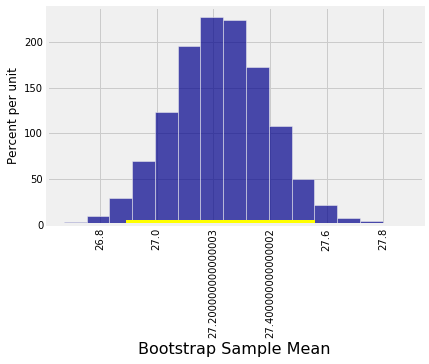
The bootstrap confidence interval is essentially identical to the interval (26.89, 27.57) that we got by using the normal approximation.

As we did in Data 8, let’s observe that the distribution of maternal ages in the sample is far from normal:

baby.select('Maternal Age').hist()

png

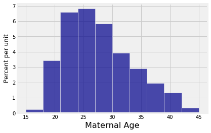
But the empirical distribution of the sample mean, displayed as the output of the previous cell, is roughly bell shaped. That is because the probability distribution of the mean of the large sample is approximately normal by the Central Limit Theorem, even though the distribution of the population is skewed.