Independence

Interact

Jointly distributed random variables $X$ and $Y$ are independent if $P(X \in A, Y \in B) = P(X \in A)P(Y \in B)$ for all intervals $A$ and $B$ .

Let $X$ have density $f_X$ , let $Y$ have density $f_Y$ , and suppose $X$ and $Y$ are independent. Then if $f$ is the joint density of $X$ and $Y$ ,

$\begin{align*} f(x, y)dxdy &\sim P(X \in dx, Y \in dy) \\ &= P(X \in dx)P(Y \in dy) ~~~~~ \text{(independence)} \\ &= f_X(x)dx f_Y(y)dy \\ &= f_X(x)f_Y(y)dxdy \end{align*}$

Thus if $X$ and $Y$ are independent then their joint density is given by

$f(x, y) = f_X(x)f_Y(y)$

This is the product rule for densities: the joint density of two independent random variables is the product of their densities.

Independent Standard Normal Random Variables

Suppose $X$ and $Y$ are i.i.d. standard normal random variables. Then their joint density is given by

$f(x, y) = \frac{1}{\sqrt{2\pi}} e^{-\frac{1}{2}x^2} \cdot \frac{1}{\sqrt{2\pi}} e^{-\frac{1}{2}y^2}, ~~~~ -\infty < x, y < \infty$

Equivalently, $f(x, y) = \frac{1}{2\pi} e^{-\frac{1}{2}(x^2 + y^2)}, ~~~~ -\infty < x, y < \infty$

Here is a graph of the joint density surface.

def indep_standard_normals(x,y):
    return 1/(2*math.pi) * np.exp(-0.5*(x**2 + y**2))

Plot_3d((-4, 4), (-4, 4), indep_standard_normals, rstride=4, cstride=4)

png

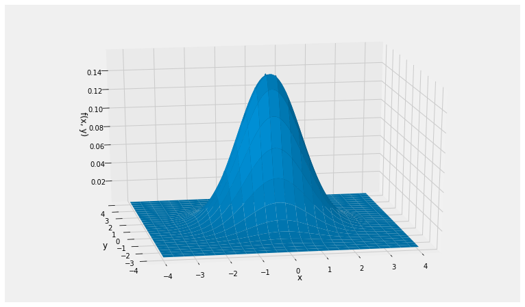
Notice the circular symmetry of the surface. This is because the formula for the joint density involves the pair $(x, y)$ through the expression $x^2 + y^2$ which is symmetric in $x$ and $y$ .

Notice also that $P(X = Y) = 0$ , as the probability is the volume over a line. This is true of all pairs of independent random variables with a joint density: $P(X = Y) = 0$ . So for example $P(X > Y) = P(X \ge Y)$ . You don’t have to worry about whether or not to the inequality should be strict.

The Larger of Two Independent Exponential Random Variables

Let $X$ and $Y$ be independent random variables. Suppose $X$ has the exponential $(\lambda)$ distribution and $Y$ has the exponential $(\mu)$ distribution. The goal of this example is to find $P(Y > X)$ .

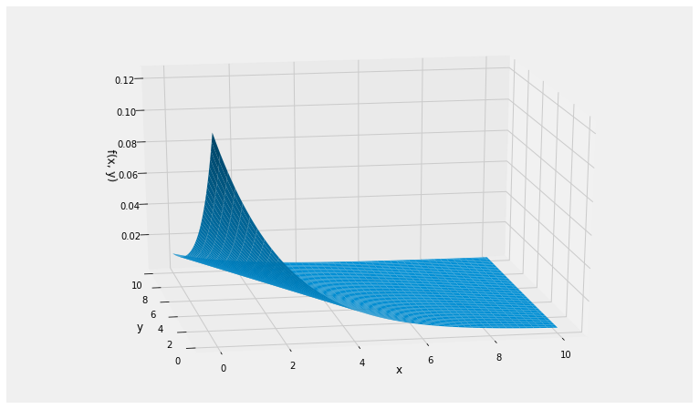
By the product rule, the joint density of $X$ and $Y$ is given by

$f(x, y) ~ = ~ \lambda e^{-\lambda x} \mu e^{-\mu y}, ~~~~ x > 0, ~ y > 0$

The graph below shows the joint density surface in the case $\lambda = 0.5$ and $\mu = 0.25$ , so that $E(X) = 2$ and $E(Y) = 4$ .

def independent_exp(x, y):
    return 0.5 * 0.25 * np.e**(-0.5*x - 0.25*y)

Plot_3d((0, 10), (0, 10), independent_exp)

png

To find $P(Y > X)$ we must integrate the joint density over the upper triangle of the first quadrant, a portion of which is shown below.

png

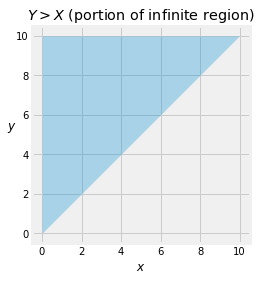
The probability is therefore $P(Y > X) ~ = ~ \int_0^\infty \int_x^\infty \lambda e^{-\lambda x} \mu e^{-\mu y} dy dx$

We can do this double integral without much calculus, just by using probability facts.

$\begin{align*} P(Y > X) &= \int_0^\infty \int_x^\infty \lambda e^{-\lambda x} \mu e^{-\mu y} dy dx \\ \\ &= \int_0^\infty \lambda e^{-\lambda x} \big{(} \int_x^\infty \mu e^{-\mu y} dy\big{)} dx \\ \\ &= \int_0^\infty \lambda e^{-\lambda x} e^{-\mu x} dx ~~~~~~ \text{(survival function of } Y\text{, evaluated at } x \text{)} \\ \\ &= \frac{\lambda}{\lambda + \mu} \int_0^\infty (\lambda + \mu) e^{-(\lambda + \mu)x} dx \\ \\ &= \frac{\lambda}{\lambda + \mu} ~~~~~~~ \text{(total integral of exponential } (\lambda + \mu) \text{ density is 1)} \end{align*}$

Thus

$P(Y > X) ~ = ~ \frac{\lambda}{\lambda + \mu}$

Analogously,

$P(X > Y) ~ = ~ \frac{\mu}{\lambda + \mu}$

Notice that the two chances are proportional to the parameters. This is consistent with intuition if you think of $X$ and $Y$ as two lifetimes. If $\lambda$ is large, the corresponding lifetime $X$ is likely to be short, and therefore $Y$ is likely to be larger than $X$ as the formula implies.

If $\lambda = \mu$ then $P(Y > X) = 1/2$ which you can see by symmetry since $P(X = Y) = 0$ .

If we had attempted the double integral in the other order – first $x$ , then $y$ – we would have had to do more work. The integral is

$\int_0^\infty \int_0^y \lambda e^{-\lambda x} \mu e^{-\mu y} dx dy$

Let’s take the easy way out by using SymPy to confirm that we will get the same answer.

# Create the symbols; they are all positive

x = Symbol('x', positive=True)
y = Symbol('y', positive=True)
lamda = Symbol('lamda', positive=True)
mu = Symbol('mu', positive=True)

# Construct the expression for the joint density

f_X = lamda * exp(-lamda * x)
f_Y = mu * exp(-mu * y)
joint_density = f_X * f_Y
joint_density

$\lambda \mu e^{- \lambda x} e^{- \mu y}$

# Display the integral – first x, then y

Integral(joint_density, (x, 0, y), (y, 0, oo))

$\int_{0}^{\infty}\int_{0}^{y} \lambda \mu e^{- \lambda x} e^{- \mu y}\, dx\, dy$

# Evaluate the integral

answer = Integral(joint_density, (x, 0, y), (y, 0, oo)).doit()
answer

$1 - \frac{\mu}{\lambda \left(1 + \frac{\mu}{\lambda}\right)}$

# Confirm that it is the same 
# as what we got by integrating in the other order

simplify(answer)

$\frac{\lambda}{\lambda + \mu}$