2.5. Updating Probabilities#
Data changes minds. We might start out with a set of assumptions about how the world works, but as we gather more data, we may have to update our opinions based on what we see in the data.
Opinions can be reflected by probabilities, and these too can be updated as information comes in. In this section we will set up a method of updating probabilities given some data. We will start with an example and then we will state the method in greater generality.
2.5.1. Example: True Positives#
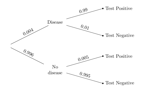
In a population there is a rare disease: only 0.4% of the people have it. There is a laboratory test for the disease that has a 99% chance of returning a positive result when run on a person that has the disease. When run on someone who doesn’t have the disease, it has a 99.5% chance of returning a negative result. So overall, it’s a pretty good test.
One person is picked at random from this population. Given that the person tests positive, what is the chance that the person has the disease?
Here is the tree diagram like the ones we drew in Data 8, to summarize the information in the problem.
To solve the problem, we will use the division rule. Let
(0.004*0.99)/(0.004*0.99 + 0.996*0.005)
0.44295302013422816
2.5.2. Bayes’ Rule#
In general, if the entire outcome space can be partitioned into events
This calculation, called Bayes’ Rule, is an application of the division rule in a setting where the events
Quick Check
You have three coins in a box. One is fair. One is biased towards heads and lands heads with chance 80%. The third is biased towards tails and lands heads with chance 10%. You pick a coin from the box at random and flip it. Given that it lands heads, what is the chance the coin is fair?
Answer
2.5.3. The Effect of the Prior#
Let’s take a closer look at the numerical value of the answer we got in our example. It’s a bit disconcerting. It says that even though the person has tested positive, there is less than 50% chance they have the disease. That seems strange, as the accuracy rates of the test are quite high.
This is not a fault of the test or of Bayes’ Rule. It’s due to our premise that the person “is picked at random from the population.” The disease is so rare that the proportion of people who have the disease and test positive is actually a bit smaller than the people who don’t have the disease and get a bad test result. This explains why the answer for a randomly picked person is less than 50%.
But people who go to get tested for a disease usually do so because they or their doctors think they should. And in that case they are no longer “randomly picked” members of the population.
For such a person, we have to rethink our assumptions about randomness. If a person thinks they might have the disease, then their subjective probability of having the disease should be larger than the probability for a random member of the population. Let’s take the following steps to see how much difference the prior makes.
We will change the “prior probability” of disease from 0.004 to other values; the prior probability of “no disease” will change correspondingly.
We will leave the test accuracy rates unchanged.
We will observe the changes in the “posterior probability” of disease given that the person tested positive, for different values of the prior.
prior = make_array(0.004, 0.01, 0.05, 0.1, 0.5)
Table().with_columns(
   'Prior P(D)', prior,
    'Posterior P(D|+)', (prior*0.99)/(prior*0.99 + (1-prior)*0.005)
)
| Prior P(D) | Posterior P(D|+) |
|---|---|
| 0.004 | 0.442953 |
| 0.01 | 0.666667 |
| 0.05 | 0.912442 |
| 0.1 | 0.956522 |
| 0.5 | 0.994975 |
The table shows that the posterior chance that the person has the disease, given that they tested positive, depends heavily on the prior. For example, if the person thinks they even have a 10% chance of the disease, then, given that they test positive, their probability of having the disease gets updated to over 95%.