The Binomial Distribution

6.1. The Binomial Distribution#

Let $X_{1}, X_{2}, \dots, X_{n}$ be i.i.d. Bernoulli $(p)$ random variables and let $S_{n} = X_{1} + X_{2} \dots + X_{n}$ . That’s a formal way of saying:

Suppose you have a fixed number $n$ of success/failure trials; and
the trials are independent; and
on each trial, the probability of success is $p$ .
Let $S_{n}$ be the total number of successes.

The first goal of this section is to find the distribution of $S_{n}$ .

In our earlier example, we were counting the number of sixes in 7 rolls of a die. The 7 rolls are independent of each other, the chance of “success” (getting a six) is $1 / 6$ on each trial, and $S_{7}$ is the number of sixes.

The first step in finding the distribution of any random variable is to identify the possible values of the variable. In $n$ trials, the smallest number of successes you can have is 0 and the largest is $n$ . So the set of possible values of $S_{n}$ is ${0, 1, 2, \dots, n}$ .

Thus the number of sixes in 7 rolls can be any integer in the 0 through 7 range. Let’s find $P (S_{7} = 3)$ .

Partition the event ${S_{7} = 3}$ into the different ways it can happen. One way can be denoted SSSFFFF, where S denotes “success” (or “six”), and F denotes failure. Another is SFFSSFF. And so on.

Now notice that

P (SSSFFFF) = (\frac{1}{6})^{3} (\frac{5}{6})^{4} = P (SFFSSFF)

by independence. Indeed, any sequence of three S’s and four F’s has the same probability. So by the addition rule,

\begin{array}{r} \begin{aligned} P (S_{7} = 3) & = (number of sequences that have three S and four F) \cdot (\frac{1}{6})^{3} (\frac{5}{6})^{4} \\ = (\binom{7}{3}) (\frac{1}{6})^{3} (\frac{5}{6})^{4} \end{aligned} \end{array}

because $(\binom{7}{3})$ counts the number of ways you can choose 3 places out of 7 in which to put the symbol S, with the remaining 4 places being filled with F.

An analogous argument leads us to one of the most important distributions in probability theory.

6.1.1. The Binomial $(n, p)$ Distribution#

Let $S_{n}$ be the number of successes in $n$ independent Bernoulli $(p)$ trials. Then $S_{n}$ has the binomial distribution with parameters $n$ and $p$ , defined by

P (S_{n} = k) = (\binom{n}{k}) p^{k} (1 - p)^{n - k}, k = 0, 1, \dots, n

Parameters of a distribution are constants associated with it. The Bernoulli $(p)$ distribution has parameter $p$ . The binomial distribution defined above has parameters $n$ and $p$ and is referred to as the binomial $(n, p)$ distribution for short. You should check that the Bernoulli $(p)$ distribution is the same as the binomial $(1, p)$ distribution.

Before we get going on calculations with the binomial distribution, let’s make a few observations.

The functional form of the probabilities is symmetric in successes and failures, because

P (S_{n} = k) = \frac{n!}{k! (n - k)!} p^{k} (1 - p)^{n - k}, k = 0, 1, \dots, n

That’s “number of trials factorial; divided by number of successes factorial times number of failures factorial; times the probability of success to the power number of successes; times the probability of failure to the power number of failures.”

The formula makes sense for the edge cases $k = 0$ and $k = n$ . We can calculate $P (S_{n} = 0)$ without any of the machinery developed above. It’s the chance of no successes, which is the chance of all failures, which is $(1 - p)^{n}$ . Our formula says

P (S_{n} = 0) = \frac{n!}{0! (n - 0)!} p^{0} (1 - p)^{n - 0} = (1 - p)^{n}

after all the dust clears in the formula; the first two factors are both 1. You can check that $P (S_{n} = n) = p^{n}$ , the chance that all the trials are successes.

Remember that $0! = 1$ by definition. In part, it is defined that way to make the formula for $(\binom{n}{k})$ work out correctly when $k = 0$ .

The probabilities in the distribution sum to 1. To see this, recall that for any two numbers $a$ and $b$ ,

\begin{array}{r} \begin{aligned} (a + b)^{2} & = a^{2} + 2 a b + b^{2} \\ (a + b)^{3} & = a^{3} + 3 a^{2} b + 3 a b^{2} + b^{3} \\ \dots \\ (a + b)^{n} & = \sum_{k = 0}^{n} (\binom{n}{k}) a^{k} b^{n - k} \end{aligned} \end{array}

by the binomial expansion of $(a + b)^{n}$ . The numbers $(\binom{n}{k})$ are the elements of Pascal’s triangle, as you will have seen in a math class, and are called binomial coefficients.

Plug in $a = p$ and $b = 1 - p$ and notice that the terms in the sum are exactly the binomial probabilities we defined above. So the sum of the probabilities is

\sum_{k = 0}^{n} (\binom{n}{k}) p^{k} (1 - p)^{n - k} = (p + (1 - p))^{n} = 1^{n} = 1

6.1.2. Applying the Formula#

To use the binomial formula, you first have to recognize that it can be used, and then use it as you would use any distribution.

Check the conditions: a known number of independent, repeated, success/failure trials, and you are counting the number of successes
Identify the two parameters $n$ and $p$
Identify each $k$ for which the event occurs
Add up the binomial $(n, p)$ probabilities for all $k$ in the set you identified (or, if the set is very large, add up the probabilities in the complement and then subtract from 1)

Quick Check

Every time I throw a dart, I have chance 25% of hitting the bullseye, independent of all other throws. Suppose I throw the dart 10 times. Find the chance that

(a) I hit the bullseye two times

(b) I hit the bullseye more than two times

(c) I hit the bullseye more than six times

Answer

(a) $(\binom{10}{2}) {0.25}^{2} {0.75}^{8}$

(b) $1 - \sum_{k = 0}^{2} (\binom{10}{k}) {0.25}^{k} {0.75}^{10 - k}$

(c) $\sum_{k = 7}^{10} (\binom{10}{k}) {0.25}^{k} {0.75}^{10 - k}$

6.1.3. Binomial Probabilities in Python#

SciPy is a system for scientific computing, based on Python. The stats submodule of scipy does numerous calculations in probability and statistics. We will be importing it at the start of every notebook from now on.

from scipy import stats

The function stats.binom.pmf takes three arguments: $k$ , $n$ , and $p$ , in that order. It returns the numerical value of $P (S_{n} = k)$ For short, we will say that the function returns the binomial $(n, p)$ probability of $k$ .

The acronym “pmf” stands for probability mass function which as we have noted earlier is sometimes used as another name for the distribution of a variable that has finitely many values.

The chance of 3 sixes in 7 rolls of a die is $(\binom{7}{3}) (1 / 6)^{3} (5 / 6)^{4}$ by the binomial formula, which works out to about 8% by the calculation below.

stats.binom.pmf(3, 7, 1/6)

0.078142861225423008

You can also specify an array or list of values of $k$ , and stats.binom.pmf will return an array consisting of all their probabilities.

stats.binom.pmf([2, 3, 4], 7, 1/6)

array([ 0.23442858,  0.07814286,  0.01562857])

Thus to find $P (2 \leq S_{7} \leq 4)$ , you can use

sum(stats.binom.pmf([2, 3, 4], 7, 1/6))

0.32820001714677643

6.1.4. Cumulative Distribution Function (cdf)#

To visualize binomial distributions we will use the prob140 method Plot, by first using stats.binom.pmf to calculate the binomial probabilities. The cell below plots the distribution of $S_{7}$ above. Notice how we start by specifying all the possible values of $S_{7}$ in the array k.

n = 7
p = 1/6
k = np.arange(n+1)
binom_7_1_6 = stats.binom.pmf(k, n, p)
binom_7_1_6_dist = Table().values(k).probabilities(binom_7_1_6)
Plot(binom_7_1_6_dist)

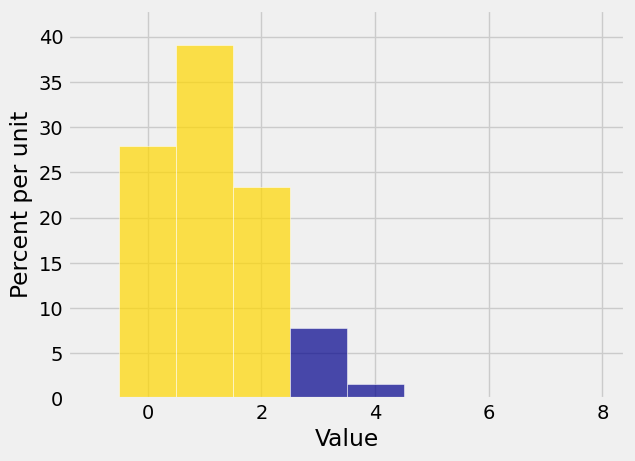
../../_images/7baa4ab642b6080d37c5f58e1a4080670f4a1efdfa5668df108ff15cfd42d030.png

Very often, we need probabilities of the form $P (X > x)$ or $P (X \leq x)$ . For example, for $X$ with the binomial $(7, 1 / 6)$ distribution above, here is the event ${X \leq 2}$ .

Plot(binom_7_1_6_dist, event=np.arange(0, 3))

../../_images/61235dd2116fdb251f7e3d59b6c6ee4fb74b49c0505f5ad4bd5851a5dd9ed8c2.png

The cumulative distribution function or c.d.f. of any random variable is a function that calculates this “area to the left” of any point. If you denote the c.d.f. by $F$ , then

F (x) = P (X \leq x)

for any x.

We will get to know this function better later in the course. For now, note that stats lets you calculate it directly without having to use pmf and then summing. The function is called stats.distribution_name.cdf where distribution_name could be binom or hypergeom or any other distribution name that stats recognizes. The first argument is $x$ , followed by the parameters of the distribution in a specified order.

For $X$ a binomial $(7, 1 / 6)$ random variable, the gold area above is $F (2)$ which is about 90.4%.

To find $P (X > 2)$ , we can use the cdf again:

P (X > 2) = 1 - P (X \leq 2) = 1 - F (2)

1 - stats.binom.cdf(2, 7, 1/6)

0.095775462962963021

stats.binom.cdf(2, 7, 1/6)

0.90422453703703698

Here is the event $P (5 < Y \leq 10)$ for a random variable $Y$ that has the binomial $(20, 0.4)$ distribution.

k = np.arange(21)
probs = stats.binom.pmf(k, 20, 0.4)
binom_20_point4 = Table().values(k).probabilities(probs)
Plot(binom_20_point4, event=np.arange(6, 11))

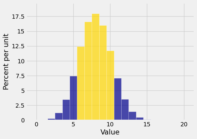
../../_images/9fba67c2f56391039a13378592c93a14b0fba3ab51cff9b21bc36bec2f16c036.png

To find $P (5 < Y \leq 10)$ we can sum the areas of the gold bars. But we can also use the cdf:

P (5 < Y \leq 10) = P (Y \leq 10) - P (Y \leq 5)

That’s about 74.7%.

stats.binom.cdf(10, 20, 0.4) - stats.binom.cdf(5, 20, 0.4)

0.74687978112974585

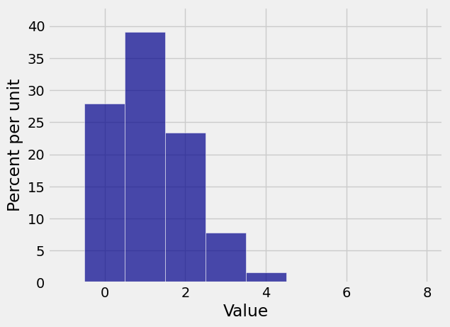
6.1.5. Binomial Histograms#

Here is the histogram of the binomial $(7, 1 / 6)$ distribution again. Not surprisingly, the graph shows that in 7 rolls of a die you are most likely to get around 1 six.

Plot(binom_7_1_6_dist)

This distribution is not symmetric, as you would expect. But something interesting happens to the distribution of the number of sixes when you increase the number of rolls.

n = 600
p = 1/6
k = np.arange(n+1)
binom_600_1_6 = stats.binom.pmf(k, n, p)
binom_600_1_6_dist = Table().values(k).probabilities(binom_600_1_6)
Plot(binom_600_1_6_dist)

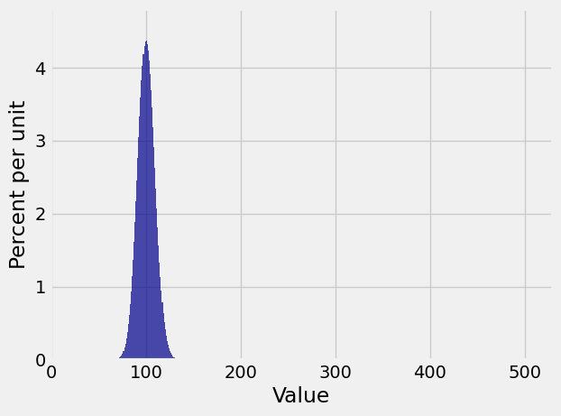
../../_images/59aee24f934f83181c7b12c45b65a7cb5b612aec08933285c36bacd9a90cf134.png

This distribution is close to symmetric, even though the die has only a 1/6 chance of showing a six.

Also notice that while the the possible values of the number of sixes range from 0 to 600, the probable values are in a much smaller range. The plt.xlim function allows us to zoom in on the probable values. The semicolon is just to prevent Python giving us a message that clutters up the graph. The edges=True option forces Plot to draw lines separating the bars; by default, it stops doing that if the number of bars is large.

Plot(binom_600_1_6_dist, edges=True)
plt.xlim(70, 130);

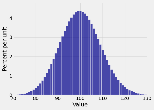
../../_images/eeb546a7c301f3187fe4c3fd7cf6448e34434a6ef7945178efd5e580f762d8e4.png

But the binomial $(n, p)$ distribution doesn’t always look bell shaped if $n$ is large.

Something quite different happens if for example your random variable is the number of successes in 600 independent trials that have probability 1/600 of success on each trial. Then the distribution of the number of successes is binomial $(600, 1 / 600)$ , which looks like this:

n = 600
p = 1/600
k = np.arange(n+1)
binom_600_1_600 = stats.binom.pmf(k, n, p)
binom_600_1_600_dist = Table().values(k).probabilities(binom_600_1_600)
Plot(binom_600_1_600_dist)

../../_images/1c55dfcfee955b01a772fc71c379e922bc1f16ec49ea4d845342de3892eb7d59.png

We really can’t see that at all! Let’s zoom in. When we set the limits on the horizontal axis, we have to account for the bar at 0 being centered at the 0 and hence starting at -0.5.

Plot(binom_600_1_600_dist, edges=True)
plt.xlim(-1, 10);

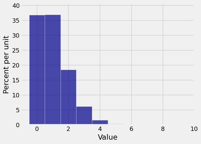
../../_images/d6d938f5581ee3ad4f091d1398c07ddbbfe5a78e12cbd6f1912e56f684cb613f.png

Now you can see that in 600 independent trials with probability 1/600 of success on each trial, you are most likely to get no successes or 1 success. There is some chance that you get 2 through 4 successes, but the chance of any number of successes greater than 4 is barely visible on the scale of the graph.

Clearly, the shape of the histogram is determined by both $n$ and $p$ . We will study the shape carefully in an upcoming section. But first let’s see some numerical examples of using the binomial distribution.