18.4. Chi-Squared Distributions

The gamma family has two important branches. The first consists of gamma \((r, \lambda)\) distributions with integer shape parameter \(r\), as you saw in the previous section.

The other important branch consists of gamma \((r, \lambda)\) distributions that have half-integer shape parameter \(r\), that is, when \(r = n/2\) for a positive integer \(n\). Notice that this branch contains the one above: every integer \(r\) is also half of the integer \(n = 2r\).

18.4.1. Chi-Squared \((1)\)

We have already seen the fundamental member of the branch. Let \(Z\) be a standard normal random variable and let \(V = Z^2\). By the change of variable formula for densities, we found the density of \(V\) to be

\[ f_V(v) ~ = ~ \frac{1}{\sqrt{2\pi}} v^{-\frac{1}{2}} e^{-\frac{1}{2} v}, ~~~~ v > 0 \]

That’s the gamma \((1/2, 1/2)\) density. It is also called the chi-squared density with 1 degree of freedom, which we will abbreviate to chi-squared (1).

See More

18.4.2. From Chi-Squared \((1)\) to Chi-Squared \((n)\)

When we were establishing the properties of the standard normal density, we discovered that if \(Z_1\) and \(Z_2\) are independent standard normal then \(Z_1^2 + Z_2^2\) has the exponential \((1/2)\) distribution. We saw this by comparing two different settings in which the Rayleigh distribution arises. But that wasn’t a particularly illuminating reason for why \(Z_1^2 + Z_2^2\) should be exponential.

But now we know that the sum of independent gamma variables with the same rate is also gamma; the shape parameter adds up and the rate remains the same. Therefore \(Z_1^2 + Z_2^2\) is a gamma \((1, 1/2)\) variable. That’s the same distribution as exponential \((1/2)\), as you showed in exercises. This explains why the sum of squares of two i.i.d. standard normal variables has the exponential \((1/2)\) distribution.

If \(Z_1, Z_2, Z_3\) are i.i.d. standard normal variables, then:

• \(Z_1^2\) has the gamma \((1/2, 1/2)\) distribution

• \(Z_1^2 + Z_2^2\) has the gamma \((1/2 + 1/2, 1/2)\) distribution

• \(Z_1^2 + Z_2^2 + Z_3^2\) has the gamma \((1/2 + 1/2 + 1/2, 1/2)\) distribution

Now let \(Z_1, Z_2, \ldots, Z_n\) be i.i.d. standard normal variables. Then \(Z_1^2, Z_2^2, \ldots, Z_n^2\) are i.i.d. chi-squared \((1)\) variables. That is, each of them has the gamma \((1/2, 1/2)\) distribution.

By induction, \(Z_1^2 + Z_2^2 + \cdots + Z_n^2\) has the gamma \((n/2, 1/2)\) distribution. This is called the chi-squared distribution with \(n\) degrees of freedom, which we will abbreviate to chi-squared \((n)\).

In data science, these distributions often arise when we work with the sum of squares of normal errors. This is usually part of a mean squared error calculation.

18.4.3. Chi-Squared Distribution with \(n\) Degrees of Freedom

For a positive integer \(n\), the random variable \(X\) has the chi-squared distribution with \(n\) degrees of freedom if the distribution of \(X\) is gamma \((n/2, 1/2)\). That is, \(X\) has density

\[ f_X(x) ~ = ~ \frac{\frac{1}{2}^{\frac{n}{2}}}{\Gamma(\frac{n}{2})} x^{\frac{n}{2} - 1} e^{-\frac{1}{2}x}, ~~~~ x > 0 \]

Here are the graphs of the chi-squared densities for degrees of freedom 2 through 5.

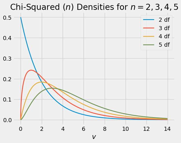
The chi-squared (2) distribution is exponential because it is the gamma \((1, 1/2)\) distribution. This distribution has three names:

• chi-squared (2)

• gamma (1, 1/2)

• exponential (1/2)

18.4.4. Mean and Variance

You know that if \(T\) has the gamma \((r, \lambda)\) density then

\[ E(T) ~ = ~ \frac{r}{\lambda} ~~~~~~~~~~~~ SD(T) = \frac{\sqrt{r}}{\lambda} \]

If \(X\) has the chi-squared \((n)\) distribution then \(X\) is gamma \((n/2, 1/2)\). So

\[ E(X) ~ = ~ \frac{n/2}{1/2} ~ = ~ n \]

Thus the expectation of a chi-squared random variable is its degrees of freedom.

The SD is

\[ SD(X) ~ = ~ \frac{\sqrt{n/2}}{1/2} ~ = ~ \sqrt{2n} \]

18.4.5. Estimating the Normal Variance

Suppose \(X_1, X_2, \ldots, X_n\) are i.i.d. normal \((\mu, \sigma^2)\) variables, and that you are in a setting in which you know \(\mu\) and are trying to estimate \(\sigma^2\).

Let \(Z_i\) be \(X_i\) in standard units, so that \(Z_i = (X_i - \mu)/\sigma\). Define the random variable \(T\) as follows:

\[ T ~ = ~ \sum_{i=1}^n Z_i^2 ~ = ~ \frac{1}{\sigma^2}\sum_{i=1}^n (X_i - \mu)^2 \]

Then \(T\) has the chi-squared \((n)\) distribution and \(E(T) = n\). Now define \(W\) by

\[ W ~ = ~ \frac{\sigma^2}{n} T ~ = ~ \frac{1}{n} \sum_{i=1}^n (X_i - \mu)^2 \]

Then \(W\) can be computed based on the sample since \(\mu\) is known. And since \(W\) is a linear tranformation of \(T\) it is easy to see that \(E(W) = \sigma^2\).

So we have constructed an unbiased estimate of \(\sigma^2\). It is the mean squared deviation from the known population mean.

But typically, \(\mu\) is not known. In that case you need a different estimate of \(\sigma^2\) since you can’t compute \(W\) as defined above. You showed in exercises that

\[ S^2 ~ = ~ \frac{1}{n-1}\sum_{i=1}^n (X_i - \bar{X})^2 \]

is an unbiased estimate of \(\sigma^2\) regardless of the distribution of the \(X_i\)’s. When the \(X_i\)’s are normal, as is the case here, it turns out that \(S^2\) is a linear transformation of a chi-squared \((n-1)\) random variable. We will show that later in the course.

18.4.6. “Degrees of Freedom”

The example above helps explain the strange term “degrees of freedom” for the parameter of the chi-squared distribution.

• When \(\mu\) is known, you have \(n\) independent centered normals \((X_i - \mu)\) that you can use to estimate \(\sigma^2\). That is, you have \(n\) degrees of freedom in constructing your estimate.

• When \(\mu\) is not known, you are using all \(n\) of \(X_1 - \bar{X}, X_2 - \bar{X}, \ldots, X_n - \bar{X}\) in your estimate, but they are not independent. They are the deviations of the list \(X_1, X_2, \ldots , X_n\) from their average \(\bar{X}\), and hence their sum is 0. If you know \(n-1\) of them, the final one is determined. So you only have \(n-1\) degrees of freedom.