12.2. Prediction and Estimation#

One way to think about the SD is in terms of errors in prediction. Suppose I am going to generate a value of the random variable \(X\), and I ask you to predict the value I am going to get. What should you use as your predictor?

A natural choice is \(\mu_X\), the expectation of \(X\). But you could choose any number \(c\). The error that you will make is \(X - c\). About how big is that? For most reasonable choices of \(c\), the error will sometimes be positive and sometimes negative. To find the rough size of this error, we will avoid cancellation as before, and start by calculating the mean squared error of the predictor \(c\):

\[ MSE(c) ~ = ~ E[(X-c)^2] \]

Notice that by definition, the variance of \(X\) is the mean squared error of using \(\mu_X\) as the predictor.

\[ MSE(\mu_X) ~ = ~ E[(X-\mu_X)^2] ~ = ~ \sigma_X^2 \]

We will now show that \(\mu_X\) is the least squares constant predictor, that is, it has the smallest mean squared error among all constant predictors. Since we have guessed that \(\mu_X\) is the best choice, we will organize the algebra around that value.

\[\begin{split} \begin{align*} MSE(c) ~ = ~ E\big{[}(X - c)^2\big{]} &= E\big{[} \big{(} (X - \mu_X) + (\mu_X - c) \big{)}^2 \big{]} \\ &= E\big{[} (X - \mu_X)^2 \big{]} +2(\mu_X - c)E\big{[} (X-\mu_X) \big{]} + (\mu_X -c)^2 \\ &= \sigma_X^2 + 0 + (\mu_X -c)^2 \\ &\ge \sigma_X^2 \\ &= MSE(\mu_X) \end{align*} \end{split}\]

with equality if and only if \(c = \mu_X\).

12.2.1. The Mean as a Least Squares Predictor#

What we have shown is the predictor \(\mu_X\) has the smallest mean squared error among all choices \(c\). That smallest mean squared error is the variance of \(X\), and hence the smallest root mean squared error is the SD \(\sigma_X\).

This is why a common approach to prediction is, “My guess is the mean, and I’ll be off by about an SD.”

Quick Check

Your friend has a random dollar amount \(X\) in their wallet. Suppose you know that \(E(X) = 16\) dollars and \(SD(X) = 3\) dollars. In all your answers below, please include units of measurement.

(a) What is the least squares constant predictor of \(X\)?

(b) What is the mean squared error of this predictor?

(c) What is the root mean squared error of this predictor?

12.2.2. German Tanks, Revisited#

Recall the German tanks problem in which we have a sample \(X_1, X_2, \ldots , X_n\) drawn at random without replacement from \(1, 2, \ldots , N\) for some fixed \(N\), and we are trying to estimate \(N\).

We came up with two unbiased estimators of \(N\):

  • An estimator based on the sample mean: \(T_1 = 2\bar{X}_n - 1\) where \(\bar{X}_n\) is the sample average \(\frac{1}{n}\sum_{i=1}^n X_i\)

  • An estimator based on the sample maximum: \(T_2 = M\cdot\frac{n+1}{n} - 1\) where \(M = \max(X_1, X_2, \ldots, X_n)\).

Here are simulated distributions of \(T_1\) and \(T_2\) in the case \(N = 300\) and \(n = 30\), based on 5000 repetitions.

def simulate_T1_T2(N, n):
    """Returns one pair of simulated values of T_1 and T_2
    based on the same simple random sample"""
    tanks = np.arange(1, N+1)
    sample = np.random.choice(tanks, size=n, replace=False)
    t1 = 2*np.mean(sample) - 1
    t2 = max(sample)*(n+1)/n - 1
    return [t1, t2]

def compare_T1_T2(N, n, repetitions):
    """Returns a table of simulated values of T_1 and T_2, 
    with the number of rows = repetitions
    and each row containing the two estimates based on the same simple random sample"""
    tbl = Table(['T_1 = 2*Mean-1', 'T_2 = Augmented Max'])
    for i in range(repetitions):
        tbl.append(simulate_T1_T2(N, n))
    return tbl

N = 300
n = 30
repetitions = 5000
comparison = compare_T1_T2(N, n, 5000)   
comparison.hist(bins=np.arange(N/2, 3*N/2))
plt.title('$N =$'+str(N)+', $n =$'+str(n)+' ('+str(repetitions)+' repetitions)');
../../_images/02_Prediction_and_Estimation_9_0.png

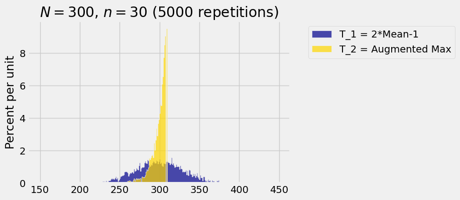
We know that both estimators are unbiased: \(E(T_1) = N = E(T_2)\). But is clear from the simulation that \(SD(T_1) > SD(T_2)\) and hence \(T_2\) is a better estimator than \(T_1\).

The empirical values of the two means and standard deviations based on this simulation are calculated below.

t1 = comparison.column(0)
np.mean(t1), np.std(t1)
(300.05885333333333, 30.148536538218014)
t2 = comparison.column(1)
np.mean(t2), np.std(t2)
(300.11209333333335, 9.070651475816568)

These standard deviations are calculated based on empirical data given a specified value of the parameter \(N = 300\) and a specified sample size \(n = 30\). In the next chapter we will develop properties of the SD that will allow us to obtain algebraic expressions for \(SD(T_1)\) and \(SD(T_2)\) for all \(N\) and \(n\).