5.1. Bounding the Chance of a Union#
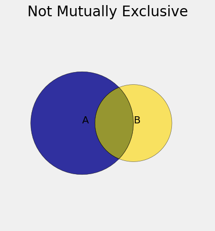
Before we get to larger collections of events, let’s consider the union of two events that are not mutually exclusive. The diagram below shows two such events. The union is the entire colored region: the blue, the gold, as well as the intersection.
An exercise in an early chapter asks you to use additivity to show that
One of the pieces of the formula is the chance of the intersection. If the nature of the dependence between
Keep in mind that bounds aren’t approximations. They might be quite far off the exact value.
Keep in mind also that bounds on the chance of a union can be manipulated to become bounds on the chance of an intersection.
The union of a collection of events is that event that at least one of them occurs.
The complement of the union is the event that none of them occurs, that is, the event that all of them don’t occur.
If the chance of a union is at most
See More
5.1.1. Boole’s Inequality#
For
For now, we’ll observe something much simpler, which is that adding the probabilities of all the individual events and not dealing with the overlaps must give us an upper bound on the chance of the union.
You can see that in the diagram above, for
Boole’s Inequality provides an upper bound on the chance of the union of
That is, the chance that at least one of the events occurs can be no larger than the sum of the chances.
We have discussed why the inequality is true for
Because
So
For example, if the weather forecast says that the chance of rain on Saturday is 40% and the chance of rain on Sunday is 10%, then the chance that it rains at some point during those two days is at least 40% and at most 50%.
To find the chance exactly, you would need the chance that it rains on both days, which you don’t have. Assuming independence doesn’t seem like a good idea in this setting. So you cannot compute an exact answer, and must be satisfied with bounds.
Quick Check
In a class, 60% of the students have read The Merchant of Venice and 10% have read Hamlet. Fill in the blanks with the best bounds you can find based on the information given.
(a) The chance that a randomly picked student has read at least one of the two plays is at least
(b) The chance that a randomly picked student has read neither of the two plays is at least
Answer
(a) 60%, 70%
(b) 30%, 40%
Though bounds aren’t exact answers or even approximations, they can be very useful. Here is an example of a common use of Boole’s Inequality in data science. It has Bonferroni’s name attached to it, because Boole and Bonferroni both have related bounds on probabilities of unions.
5.1.2. Bonferroni Method#
Suppose you are estimating five parameters based on a random sample, and that for each parameter you have a method that produces a good estimate with any pre-specified chance. For example, if the estimate has to be good with chance 99%, you have a way of doing that.
Now suppose you want your estimates to be such that all five are good with chance 95%. What should you do?
It is not enough to make each estimate good with chance 95%. If you do that, the chance that they are all good will be less than 95%, because the event “all are good” is a subset of each event “Estimate
Boole’s Inequality can help you figure out what to do.
Let
You can get yourself out of this problem by looking at the complement of the event “all five are good”. The complement is “at least one is bad”, which is the union of the events “Estimate
Each term in the sum is the chance that the corresponding estimate is bad. You want those chances to be small. But you also want them to be large enough so that their sum is at least 0.05, because of the calculation above.
One way is to make each of them equal to
The Bonferroni method shows that if you construct each of five estimates so that it is good with chance 99%, then the chance that all five estimates are good will be at least 95%.
You can replace 95% by any other threshold and carry out the calculation again to see how good the individual estimates have to be so that they are simultaneously good with a chance that exceeds the threshold.