10.1. Transitions#
The state space of a process is the set of possible values of the random variables in the process. We will often denote the state space by \(S\).
For example, consider a random walk where a gambler starts with a fortune of \(a\) dollars for some positive integer \(a\), and bets on successive tosses of a fair coin. If the coin lands heads he gains a dollar, and if it lands tails he loses a dollar.
Let \(X_{0} = a\), and for \(n > 0\) let \(X_{n+1} = X_n + I_n\) where \(I_1, I_2, \ldots\) is an i.i.d. sequence of increments, each taking the value \(+1\) or \(-1\) with chance \(1/2\). The state space of this random walk \(X_0, X_1, X_2, \dots\) is the set of all integers. In this course we will restrict the state space to be discrete and typically finite.
See More
10.1.1. Markov Property#
Consider a stochastic process \(X_0, X_1, X_2, \ldots\). The Markov property formalizes the idea that the future of the process depends only on where the process is at present, not on how it got there.
For each \(n \ge 1\), the conditional distribution of \(X_{n+1}\) given \(X_0, X_1, \ldots , X_n\) depends only on \(X_n\).
That is, for every sequence of possible values \(i_0, i_1, \ldots, i_n, i_{n+1}\),
The Markov property holds for the random walk described above. Given the gambler’s fortune at time \(n\), the distribution of his fortune at time \(n+1\) doesn’t depend on his fortune before time \(n\). So the process \(X_0, X_1, X_2, \ldots \) is a Markov Chain representing the evolution of the gambler’s fortune over time.
Conditional Independence
Recall that two random variables \(X\) and \(Y\) are independent if the conditional distribution of \(X\) given \(Y\) is just the unconditional distribution of \(X\).
Random variables \(X\) and \(Y\) are said to be conditionally independent given \(Z\) if the conditional distribution of \(X\) given both \(Y\) and \(Z\) is just the conditional distribution of \(X\) given \(Z\) alone. That is, if you know \(Z\), then additional knowledge about \(Y\) doesn’t change your opinion about \(X\).
In a Markov Chain, if you define time \(n\) to be the present, time \(n+1\) to be the future, and times \(0\) through \(n-1\) to be the past, then the Markov property says that the past and future are conditionally independent given the present.
10.1.2. Initial Distribution and Transition Probabilities#
Let \(X_0, X_1, X_2, \ldots\) be a Markov chain with state space \(S\). The distribution of \(X_0\) is called the initial distribution of the chain.
A a trajectory or path is a sequence of states visited by the process. Let \(i_0 i_1 \ldots i_n\) denote a path of finite length, with \(i_j\) representing the value of \(X_j\). By the Markov property, the probability of this path is
The conditional probabilities in the product are called transition probabilities. For states \(i\) and \(j\), the conditional probability \(P(X_{n+1} = j \mid X_n = i)\) is called a one-step transition probability at time \(n\).
10.1.3. Stationary Transition Probabilities#
For many chains such as the random walk, the one-step transition probabilities depend only on the states \(i\) and \(j\), not on the time \(n\). For example, for the random walk,
for every \(n\). When one-step transition probabilites don’t depend on \(n\), they are called stationary or time-homogenous. All the Markov chains that we will study in this course have time-homogenous transition probabilities.
For such a chain, define the one-step transition probability
Then the probability of every path of finite length is the product of a term from the initial distribution and a sequence of one-step transition probabilities:
See More
10.1.4. One-Step Transition Matrix#
The one-step transition probabilities can be represented as elements of a matrix. This isn’t just for compactness of notation – it leads to a powerful theory.
The one-step transition matrix of the chain is the matrix \(\mathbb{P}\) whose \((i, j)\)th element is \(P(i, j) = P(X_1 = j \mid X_0 = i)\).
Often, \(\mathbb{P}\) is just called the transition matrix for short. Note two important properties:
\(\mathbb{P}\) is a square matrix: its rows as well as its columns are indexed by the state space.
Each row of \(\mathbb{P}\) is a distribution: for each state \(i\), and each \(n\), Row \(i\) of the transition matrix is the conditional distribution of \(X_{n+1}\) given that \(X_n = i\). Because each of its rows adds up to 1, \(\mathbb{P}\) is called a stochastic matrix.
Let’s see what the transition matrix looks like in an example.
10.1.5. Sticky Reflecting Random Walk#
Often, the transition behavior of a Markov chain is easier to describe in a transition diagram instead of a matrix. Here is such a diagram for a chain on the states 1, 2, 3, 4, and 5. The diagram shows the one-step transition probabilities.
No matter at which state the chain is, it stays there with chance 0.5.
If the chain is at states 2 through 4, it moves to each of its two adjacent state with chance 0.25.
If the chain is at states 1 or 5, it moves to its adjacent state with chance 0.5.
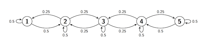
We say that there is reflection at states 1 and 5. The walk is sticky because of the positive chance of staying in place.
Transition diagrams are great for understanding the rules by which a chain moves. For calculations, however, the transition matrix is more helpful.
To start constructing the matrix, we set the array s to be the set of states and the transition function refl_walk_probs to take arguments \(i\) and \(j\) and return \(P(i, j)\).
s = np.arange(1, 6)

def refl_walk_probs(i, j):
    # staying in the same state
    if i-j == 0:
        return 0.5

    # moving left or right
    elif 2 <= i <= 4:
        if abs(i-j) == 1:
            return 0.25
        else:
            return 0

    # moving right from 1
    elif i == 1:
        if j == 2:
            return 0.5
        else:
            return 0

    # moving left from 5
    elif i == 5:
        if j == 4:
            return 0.5
        else:
            return 0
You can use the prob140 library to construct MarkovChain objects. The from_transition_function method takes two arguments:
an array of the states
a transition function
and displays the one-step transition matrix of a MarkovChain object.
reflecting_walk = MarkovChain.from_transition_function(s, refl_walk_probs)
reflecting_walk
| 1 | 2 | 3 | 4 | 5 | |
|---|---|---|---|---|---|
| 1 | 0.50 | 0.50 | 0.00 | 0.00 | 0.00 |
| 2 | 0.25 | 0.50 | 0.25 | 0.00 | 0.00 |
| 3 | 0.00 | 0.25 | 0.50 | 0.25 | 0.00 |
| 4 | 0.00 | 0.00 | 0.25 | 0.50 | 0.25 |
| 5 | 0.00 | 0.00 | 0.00 | 0.50 | 0.50 |
Compare the transition matrix \(\mathbb{P}\) with the transition diagram, and confirm that they contain the same information about transition probabilities.
To find the chance that the chain moves to \(j\) given that it is at \(i\), go to Row \(i\) and pick out the probability in Column \(j\).
Quick Check
Use the table (not the transition diagram) to find
(a) \(P(X_1 = 3 \mid X_0 = 4)\)
(b) \(P(X_{101} = 3 \mid X_{100} = 4)\)
Answer
Both answers are \(0.25\)
If you know the starting state, you can use \(\mathbb{P}\) to find the probability of any finite path. For example, given that the walk starts at 1, the probability that it then has the path [2, 2, 3, 4, 3] is
0.5 * 0.5 * 0.25 * 0.25 * 0.25
0.00390625
The MarkovChain method prob_of_path saves you the trouble of doing the multiplication. It takes as its arguments the starting state and the rest of the path (in a list or array), and returns the probability of the path given the starting state.
reflecting_walk.prob_of_path(1, [2, 2, 3, 4, 3])
0.00390625
reflecting_walk.prob_of_path(1, [2, 2, 3, 4, 3, 5])
0.0
Quick Check
Suppose the sticky reflecting walk starts at state 3. What is the chance that it then visits the states 2, 3, 3, and 4 in that order? You don’t have to simplify the product.
Answer
\(0.25 \times 0.25 \times 0.5 \times 0.25\)
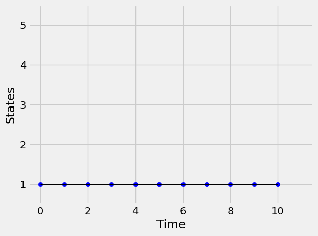
You can simulate paths of the chain using the simulate_path method. It takes two arguments: the starting state and the number of steps of the path. By default it returns an array consisting of the sequence of states in the path. The optional argument plot_path=True plots the simulated path. Run the cells below a few times and see how the output changes.
reflecting_walk.simulate_path(1, 7)
array([1, 1, 1, 1, 1, 1, 1, 2])
reflecting_walk.simulate_path(1, 10, plot_path=True)
See More
10.1.6. \(n\)-Step Transition Matrix#
For states \(i\) and \(j\), the chance of getting from \(i\) to \(j\) in \(n\) steps is called the \(n\)-step transition probability from \(i\) to \(j\). Formally, the \(n\)-step transition probability is
In this notation, the one-step transition probability \(P(i, j)\) can also be written as \(P_1(i, j)\).
The \(n\)-step transition probability \(P_n(i, j)\) can be represented as the \((i, j)\)th element of a matrix called the \(n\)-step transition matrix. For each state \(i\), Row \(i\) of the \(n\)-step transition matrix contains the distribution of \(X_n\) given that the chain starts at \(i\).
The MarkovChain method transition_matrix takes \(n\) as its argument and displays the \(n\)-step transition matrix. Here is the 2-step transition matrix of the reflecting walk defined earlier in this section.
reflecting_walk.transition_matrix(2)
| 1 | 2 | 3 | 4 | 5 | |
|---|---|---|---|---|---|
| 1 | 0.3750 | 0.5000 | 0.125 | 0.0000 | 0.0000 |
| 2 | 0.2500 | 0.4375 | 0.250 | 0.0625 | 0.0000 |
| 3 | 0.0625 | 0.2500 | 0.375 | 0.2500 | 0.0625 |
| 4 | 0.0000 | 0.0625 | 0.250 | 0.4375 | 0.2500 |
| 5 | 0.0000 | 0.0000 | 0.125 | 0.5000 | 0.3750 |
You can calculate the individual entries easily by hand. For example, the \((1, 1)\) entry is the chance of going from state 1 to state 1 in 2 steps. There are two paths that make this happen:
[1, 1, 1]
[1, 2, 1]
Given that 1 is the starting state, the total chance of the two paths is \((0.5 \times 0.5) + (0.5 \times 0.25) = 0.375\).
Quick Check
For the sticky reflecting walk, find the following if it is possible without further calculation. If it is not possible, explain why not.
(a) \(P(X_2 = 5 \mid X_0 = 3)\)
(b) \(P(X_{32} = 5 \mid X_{30} = 3)\)
Answer
Both answers are \(0.0625\)
Because of the Markov property, the one-step transition probabilities are all you need to find the 2-step transition probabilities.
In general, we can find \(P_2(i, j)\) by conditioning on where the chain was at time 1.
That’s the \((i, j)\)th element of the matrix product \(\mathbb{P} \times \mathbb{P} = \mathbb{P}^2\). Thus the 2-step transition matrix of the chain is \(\mathbb{P}^2\).
By induction, you can show that the \(n\)-step transition matrix of the chain is \(\mathbb{P}^n\). That is,
Here is a display of the 5-step transition matrix of the reflecting walk.
reflecting_walk.transition_matrix(5)
| 1 | 2 | 3 | 4 | 5 | |
|---|---|---|---|---|---|
| 1 | 0.246094 | 0.410156 | 0.234375 | 0.089844 | 0.019531 |
| 2 | 0.205078 | 0.363281 | 0.250000 | 0.136719 | 0.044922 |
| 3 | 0.117188 | 0.250000 | 0.265625 | 0.250000 | 0.117188 |
| 4 | 0.044922 | 0.136719 | 0.250000 | 0.363281 | 0.205078 |
| 5 | 0.019531 | 0.089844 | 0.234375 | 0.410156 | 0.246094 |
This is a display, but to work with the matrix we have to represent it in a form that Python recognizes as a matrix. The method get_transition_matrix does this for us. It take the number of steps \(n\) as its argument and returns the \(n\)-step transition matrix as a NumPy matrix.
For the reflecting walk, we will start by extracting \(\mathbb{P}\) as the matrix refl_walk_P.
refl_walk_P = reflecting_walk.get_transition_matrix(1)
refl_walk_P
array([[ 0.5 ,  0.5 ,  0.  ,  0.  ,  0.  ],
       [ 0.25,  0.5 ,  0.25,  0.  ,  0.  ],
       [ 0.  ,  0.25,  0.5 ,  0.25,  0.  ],
       [ 0.  ,  0.  ,  0.25,  0.5 ,  0.25],
       [ 0.  ,  0.  ,  0.  ,  0.5 ,  0.5 ]])
Let’s check that the 5-step transition matrix displayed earlier is the same as \(\mathbb{P}^5\). You can use np.linalg.matrix_power to raise a matrix to a non-negative integer power. The first argument is the matrix, the second is the power.
np.linalg.matrix_power(refl_walk_P, 5)
array([[ 0.24609375,  0.41015625,  0.234375  ,  0.08984375,  0.01953125],
       [ 0.20507812,  0.36328125,  0.25      ,  0.13671875,  0.04492188],
       [ 0.1171875 ,  0.25      ,  0.265625  ,  0.25      ,  0.1171875 ],
       [ 0.04492188,  0.13671875,  0.25      ,  0.36328125,  0.20507812],
       [ 0.01953125,  0.08984375,  0.234375  ,  0.41015625,  0.24609375]])
This is indeed the same as the matrix displayed by transition_matrix, though it is harder to read.
When we want to use \(\mathbb{P}\) in computations, we will use this matrix representation. For displays, transition_matrix is better.
10.1.7. The Long Run#
To understand the long run behavior of the chain, let \(n\) be large and let’s examine the distribution of \(X_n\) for each value of the starting state. That’s contained in the \(n\)-step transition matrix \(\mathbb{P}^n\).
Here is the display of \(\mathbb{P}^n\) for the reflecting walk, for \(n = 25, 50\), and \(100\). Keep your eyes on the rows of the matrices as \(n\) changes.
reflecting_walk.transition_matrix(25)
| 1 | 2 | 3 | 4 | 5 | |
|---|---|---|---|---|---|
| 1 | 0.129772 | 0.256749 | 0.25 | 0.243251 | 0.120228 |
| 2 | 0.128374 | 0.254772 | 0.25 | 0.245228 | 0.121626 |
| 3 | 0.125000 | 0.250000 | 0.25 | 0.250000 | 0.125000 |
| 4 | 0.121626 | 0.245228 | 0.25 | 0.254772 | 0.128374 |
| 5 | 0.120228 | 0.243251 | 0.25 | 0.256749 | 0.129772 |
reflecting_walk.transition_matrix(50)
| 1 | 2 | 3 | 4 | 5 | |
|---|---|---|---|---|---|
| 1 | 0.125091 | 0.250129 | 0.25 | 0.249871 | 0.124909 |
| 2 | 0.125064 | 0.250091 | 0.25 | 0.249909 | 0.124936 |
| 3 | 0.125000 | 0.250000 | 0.25 | 0.250000 | 0.125000 |
| 4 | 0.124936 | 0.249909 | 0.25 | 0.250091 | 0.125064 |
| 5 | 0.124909 | 0.249871 | 0.25 | 0.250129 | 0.125091 |
reflecting_walk.transition_matrix(100)
| 1 | 2 | 3 | 4 | 5 | |
|---|---|---|---|---|---|
| 1 | 0.125 | 0.25 | 0.25 | 0.25 | 0.125 |
| 2 | 0.125 | 0.25 | 0.25 | 0.25 | 0.125 |
| 3 | 0.125 | 0.25 | 0.25 | 0.25 | 0.125 |
| 4 | 0.125 | 0.25 | 0.25 | 0.25 | 0.125 |
| 5 | 0.125 | 0.25 | 0.25 | 0.25 | 0.125 |
The rows of \(\mathbb{P}^{100}\) are all the same! That means that for the reflecting walk, the distribution at time 100 doesn’t depend on the starting state. The chain has forgotten where it started.
You can increase \(n\) and see that the \(n\)-step transition matrix stays the same. By time 100, this chain has reached stationarity.
Stationarity is a remarkable property of many Markov chains, and is the main topic of this chapter.
Quick Check
Pick the correct option: If the sticky reflecting walk is run for 500 steps, the chance that it is at state 4 at time 500
(i) is about 25%.
(ii) cannot be determined or approximated because we don’t know where the chain started.
Answer
(i)