15.5. Calculus in SymPy

Working with densities involves calculus which can sometimes be time-consuming. This course gives you two ways of reducing the amount of calculus involved.

• Probabilistic methods can help reduce algebra and calculus. You’ve seen this with algebra in the discrete case. You’ll see it with calculus as we learn more about densities.

• Python has a symbolic math module called SymPy that does algebra, calculus, and much other symbolic math. In this section we will show you how to do calculus using SymPy.

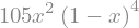
We will demonstrate the methods in the context of an example. Suppose \(X\) has density given by

\[\begin{split} f(x) = \begin{cases} 105x^2(1-x)^4 ~~~ \text{if } 0 \le x \le 1 \\ 0 ~~~~~~~~~ \text{otherwise} \end{cases} \end{split}\]

As you can see from its graph below, \(f\) could be used to model the distribution of a random proportion that you think is likely to be somewhere between 0.2 and 0.4.

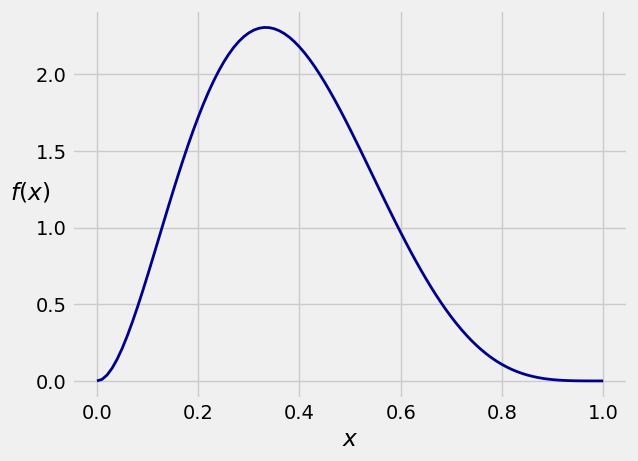
The density \(f\) is a polynomial on the unit interval, and in principle the algebra and calculus involved in integrating it are straightforward. But they are tedious. So let’s get SymPy to do the work.

First, we will import all the functions in SymPy and set up some printing methods that make the output look nicer than the retro typewritten pgf output you saw in a previous section. In future sections of this text, you can assume that this importing and initialization will have been done at the start.

from sympy import *
init_printing()

Next, we have to create tell Python that an object is symbolic. In our example, the variable \(x\) is the natural candidate to be a symbol. You can use Symbol for this, by using the argument 'x'. We have assinged the symbol to the name x.

x = Symbol('x')

Now we will assign the name density to the expression that defines \(f\). The expression looks just like a numerical calculation, but the output is algebraic!

density = 105 * x**2 * (1-x)**4
density

That’s the expression for \(f(x)\) defined by the equation at the start of the section. Notice that what we naturally think of as \(1 - x\) is expressed as \(-x + 1\). That’s because SymPy is writing the polynomial leading with the term of highest degree.

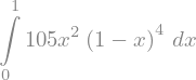
Let’s not simply accept that this function is a density. Let’s check that it is a density by integrating it from 0 to 1. To display this, we use the method Integral that takes the name of a function and a tuple (a sequence in parentheses) consisting of the variable of integration and the lower and upper limits of integration. We have assigned this integral to the name total_area.

total_area = Integral(density, (x, 0, 1))
total_area

The output of displays the integral, which is nice, but what we really want is its numerical value. In SymPy, this is achieved by abruptly instructing the method to doit().

total_area.doit()

This confirms that the function \(f\) is a density.

We can use Integral to find the chance that \(X\) is in any interval. Here is \(P(0.2 < X < 0.4)\).

prob_02_04 = Integral(density, (x, 0.2, 0.4)).doit()
prob_02_04

For \(x\) in the unit interval, the cdf of \(X\) is

\[ F(x) ~ = ~ P(X \le x) ~ = ~ \int_0^x f(s)ds ~ = ~ I(s)~ \Big{\rvert}_0^x ~ = ~ I(x) - I(0) \]

where \(I\) is the indefinite integral of \(f\).

To get the indefinite integral, simply ask SymPy to integrate the density; there are no limits of integration.

indefinite = Integral(density).doit()
indefinite

Now \(F(x) = I(x) - I(0)\). You can see at a glance that \(I(0) = 0\) but here is how SymPy would figure that out.

To evaluate \(I(0)\), SymPy must substitute \(x\) with 0 in the expression for \(I\). This is achieved by the method subs that takes the variable as its first argument and the specified value as the second.

I_0 = indefinite.subs(x, 0)
I_0

cdf = indefinite - I_0
cdf

To find the value of the cdf at a specified point, say 0.4, we have to substitute \(x\) with 0.4 in the formula for the cdf.

cdf_at_04 = cdf.subs(x, 0.4)
cdf_at_04

Thus \(P(X \le 0.4)\) is roughly 58%. Earlier we calulated \(P(0.2 < X < 0.4) = 43.2\%\), which we can confirm by using the cdf:

cdf_at_02 = cdf.subs(x, 0.2)
cdf_at_04 - cdf_at_02

The expectation \(E(X)\) is a definite integral from 0 to 1:

expectation = Integral(x*density, (x, 0, 1)).doit()
expectation

Notice how simple the answer is. Later in the course, you will see why.

Here is \(E(X^2)\), which turns out to be another simple fraction. Clearly, the density \(f\) has interesting properties. We will study them later. For now, let’s just get the numerical answers.

expected_square = Integral((x**2)*density, (x, 0, 1)).doit()
expected_square

Now you can find \(SD(X)\).

sd = (expected_square - expectation**2)**0.5
sd

15.5.1. SymPy and the Exponential Density

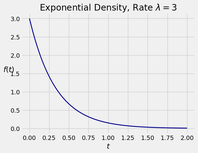
One of the primary distributions in probability theory, the exponential distribution has a positive parameter \(\lambda\) known as the “rate”, and density given by

\[ f(t) ~ = \lambda e^{-\lambda t}, ~~~ t \ge 0 \]

The density is 0 on the negative numbers. Here is its graph when \(\lambda = 3\).

To check that \(f\) is a density, we have to confirm that its integral is 1. We will start by constructing two symbols, t and lamda. Notice the incorrectly spelled lamda instead of lambda. That is because lambda has another meaning in Python, as some of you might know.

Note the use of positive=True to specify that the symbol can take on only positive values.

t = Symbol('t', positive=True)
lamda = Symbol('lamda', positive=True)

Next we construct the expression for the density. Notice the use of exp for the exponential function.

expon_density = lamda * exp(-lamda * t)
expon_density

To see that the function is a density, we can check that its integral from 0 to \(\infty\) is 1. The symbol that SymPy uses for \(\infty\) is oo, a double lower case o. It looks very much like \(\infty\).

Integral(expon_density, (t, 0, oo)).doit()

Suppose \(T\) has the exponential \((\lambda)\) density. Then for \(t \ge 0\) the cdf of \(T\) is

\[ F_T(t) ~ = ~ P(T \le t) ~ = ~ \int_0^t \lambda e^{-\lambda s}ds \]

This is a straightforward integral that you can probably do in your head. However, let’s get some more practice using SymPy to find cdf’s. We will use the same method that we used to find the cdf in the previous example.

\[ \int_0^t \lambda e^{-\lambda s}ds ~ = ~ I(t) - I(0) \]

where \(I\) is the indefinite integral of the density. To get this indefinite integral we will use Integral as before, except that this time we must specify t as the variable of integration. That is because SymPy sees two symbols t and lamda in the density, and doesn’t know which one is the variable unless we tell it.

indefinite = Integral(expon_density, t).doit()
indefinite

Now use \(F_T(t) = I(t) - I(0)\):

I_0 = indefinite.subs(t, 0)
I_0

cdf = indefinite - I_0
cdf

Thus the cdf of \(T\) is

\[ F_T(t) ~ = ~ 1 - e^{-\lambda t} \]

The expectation of \(T\) is

\[ E(T) ~ = ~ \int_0^\infty t \lambda e^{-\lambda t} dt ~ = ~ \frac{1}{\lambda} \]

which you can check by integration by parts. But SymPy is faster:

expectation = Integral(t*expon_density, (t, 0, oo)).doit()
expectation

Calculating \(E(T^2)\) is just as easy.

expected_square = Integral(t**2 * expon_density, (t, 0, oo)).doit()
expected_square

The variance and SD follow directly.

variance = expected_square - (expectation ** 2)
variance

sd = variance ** 0.5
sd

That’s a pretty funny way of writing \(\frac{1}{\lambda}\) but we’ll take it. It’s a small price to pay for not having to do all the integrals by hand.