17.2. Independence

Informally, the definition of independence is the same as before: two random variables that have a joint density are independent if additional information about one of them doesn’t change the distribution of the other.

One quick way to spot the lack of independence is to look at the set of possible values of the pair \((X, Y)\). If that set is not a rectangle then \(X\) and \(Y\) can’t be independent. The non-rectangular shape implies that there must be two values of \(X\) for which the corresponding values of \(Y\) are different.

Quick Check

The “unit disc” is the disc of radius 1 centered at the origin. That is, it’s the set of points \((x,y)\) such that \(x^2 + y^2 \le 1\). Suppose the joint density of \(X\) and \(Y\) is positive on the unit disc and \(0\) elsewhere. Pick the correct option.

(i) It is not possible to determine whether or not \(X\) and \(Y\) are independent.

(ii) \(X\) and \(Y\) are independent.

(iii) \(X\) and \(Y\) are not independent.

Answer

(iii)

See More

If the set of possible values is rectangular then you have to check independence using the old definition:

Jointly distributed random variables \(X\) and \(Y\) are independent if

\[ P(X \in A, Y \in B) = P(X \in A)P(Y \in B) \]

for all intervals \(A\) and \(B\).

Let \(X\) have density \(f_X\), let \(Y\) have density \(f_Y\), and suppose \(X\) and \(Y\) are independent. Then if \(f\) is the joint density of \(X\) and \(Y\),

\[\begin{split} \begin{align*} f(x, y)dxdy &\sim P(X \in dx, Y \in dy) \\ &= P(X \in dx)P(Y \in dy) ~~~~~ \text{(independence)} \\ &= f_X(x)dx f_Y(y)dy \\ &= f_X(x)f_Y(y)dxdy \end{align*} \end{split}\]

Thus if \(X\) and \(Y\) are independent then their joint density is given by

\[ f(x, y) = f_X(x)f_Y(y) \]

This is the product rule for densities: the joint density of two independent random variables is the product of their densities.

The converse is also true: if the joint density factors into a function of \(x\) times a function of \(y\), then \(X\) and \(Y\) are independent.

17.2.1. Independent Standard Normal Random Variables

Suppose \(X\) and \(Y\) are i.i.d. standard normal random variables. Then their joint density is given by

\[ f(x, y) = \frac{1}{\sqrt{2\pi}} e^{-\frac{1}{2}x^2} \cdot \frac{1}{\sqrt{2\pi}} e^{-\frac{1}{2}y^2}, ~~~~ -\infty < x, y < \infty \]

Equivalently,

\[ f(x, y) = \frac{1}{2\pi} e^{-\frac{1}{2}(x^2 + y^2)}, ~~~~ -\infty < x, y < \infty \]

Here is a graph of the joint density surface.

def indep_standard_normals(x,y):
    return 1/(2*math.pi) * np.exp(-0.5*(x**2 + y**2))

Plot_3d((-4, 4), (-4, 4), indep_standard_normals, rstride=4, cstride=4)

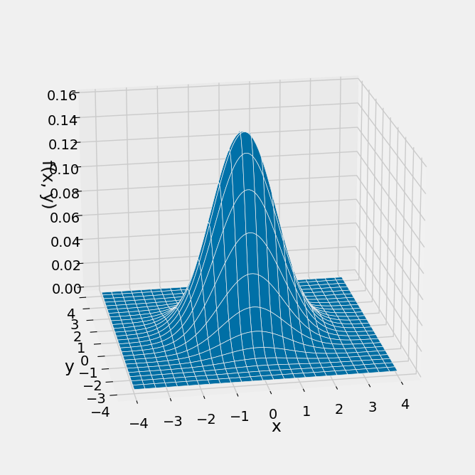
Notice the circular symmetry of the surface. This is because the formula for the joint density involves the pair \((x, y)\) through the expression \(x^2 + y^2\) which is symmetric in \(x\) and \(y\).

Notice also that \(P(X = Y) = 0\), as the probability is the volume over a line. This is true of all pairs of independent random variables with a joint density: \(P(X = Y) = 0\). So for example \(P(X > Y) = P(X \ge Y)\). You don’t have to worry about whether or not to the inequality should be strict.

Quick Check

\(X\) is normal \((0, 4)\) and \(Y\) is normal \((0, 9)\). Suppose \(X\) and \(Y\) are independent. Find the joint density of \(X\) and \(Y\).

Answer

\(f(x,y) = \frac{1}{\sqrt{2\pi}\cdot2} e^{-\frac{1}{2}\cdot\frac{x^2}{4}} \cdot \frac{1}{\sqrt{2\pi}\cdot3} e^{-\frac{1}{2}\cdot\frac{y^2}{9}}\) for all \(x, y\)

Quick Check

For some positive constant \(c\), the random variables \(X\) and \(Y\) have joint density \(f(x,y) = ce^{-\frac{1}{10}(x^2+y^2)}\) for all \(x\) and \(y\). Are \(X\) and \(Y\) independent?

Answer

Yes

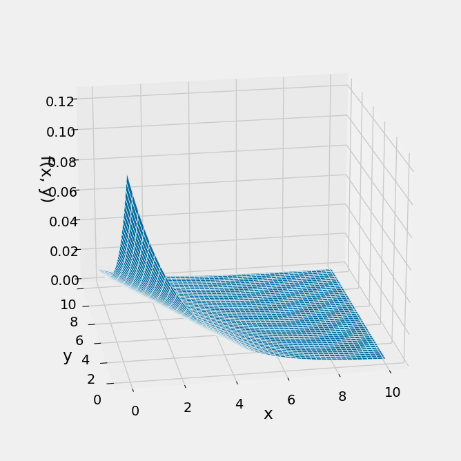
17.2.2. Competing Exponentials

Let \(X\) and \(Y\) be independent random variables. Suppose \(X\) has the exponential \((\lambda)\) distribution and \(Y\) has the exponential \((\mu)\) distribution. The goal of this example is to find \(P(Y > X)\).

By the product rule, the joint density of \(X\) and \(Y\) is given by

\[ f(x, y) ~ = ~ \lambda e^{-\lambda x} \mu e^{-\mu y}, ~~~~ x > 0, ~ y > 0 \]

The graph below shows the joint density surface in the case \(\lambda = 0.5\) and \(\mu = 0.25\), so that \(E(X) = 2\) and \(E(Y) = 4\).

def independent_exp(x, y):
    return 0.5 * 0.25 * np.e**(-0.5*x - 0.25*y)

Plot_3d((0, 10), (0, 10), independent_exp)

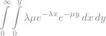
To find \(P(Y > X)\) we must integrate the joint density over the upper triangle of the first quadrant, a portion of which is shown below.

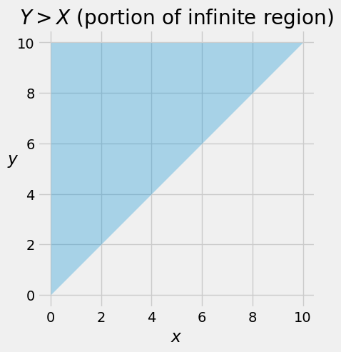
The probability is therefore

\[ P(Y > X) ~ = ~ \int_0^\infty \int_x^\infty \lambda e^{-\lambda x} \mu e^{-\mu y} dy dx \]

We can do this double integral without much calculus, just by using probability facts. As you calculate, try to involve densities as much as possible, and remember that the integral of a density over an interval is the probability of that interval.

\[\begin{split} \begin{align*} P(Y > X) &= \int_0^\infty \int_x^\infty \lambda e^{-\lambda x} \mu e^{-\mu y} dy dx \\ \\ &= \int_0^\infty \lambda e^{-\lambda x} \big{(} \int_x^\infty \mu e^{-\mu y} dy\big{)} dx \\ \\ &= \int_0^\infty \lambda e^{-\lambda x} e^{-\mu x} dx ~~~~~~ \text{(survival function of } Y\text{, evaluated at } x \text{)} \\ \\ &= \frac{\lambda}{\lambda + \mu} \int_0^\infty (\lambda + \mu) e^{-(\lambda + \mu)x} dx \\ \\ &= \frac{\lambda}{\lambda + \mu} ~~~~~~~ \text{(total integral of exponential } (\lambda + \mu) \text{ density is 1)} \end{align*} \end{split}\]

Thus

\[ P(Y > X) ~ = ~ \frac{\lambda}{\lambda + \mu} \]

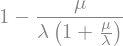
Analogously,

\[ P(X > Y) ~ = ~ \frac{\mu}{\lambda + \mu} \]

Notice that the two chances are proportional to the parameters. This is consistent with intuition if you think of \(X\) and \(Y\) as two lifetimes. If \(\lambda\) is large, the corresponding lifetime \(X\) is likely to be short, and therefore \(Y\) is likely to be larger than \(X\) as the formula implies.

If \(\lambda = \mu\) then \(P(Y > X) = 1/2\) which you can see by symmetry since \(P(X = Y) = 0\).

Quick Check

The lifetimes of two electrical components are independent. The lifetime of Component 1 has the exponential \((0.1)\) distribution, and the lifetime of Component 2 has the exponential \((0.2)\) distribution.

Without calculation, pick the correct option: The chance that Component 1 lives longer than Component 2 is

(i) greater than \(1/2\)

(ii) equal to \(1/2\)

(iii) less than \(1/2\)

Answer

(i)

Quick Check

Find the chance in Quick Check above.

Answer

\(2/3\)

If we had attempted the double integral in the other order – first \(x\), then \(y\) – we would have had to do more work. The integral is

\[ P(Y > X) ~ = ~ \int_0^\infty \int_0^y \lambda e^{-\lambda x} \mu e^{-\mu y} dx dy \]

Let’s take the easy way out by using SymPy to confirm that we will get the same answer.

# Create the symbols; they are all positive

x = Symbol('x', positive=True)
y = Symbol('y', positive=True)
lamda = Symbol('lamda', positive=True)
mu = Symbol('mu', positive=True)

# Construct the expression for the joint density

f_X = lamda * exp(-lamda * x)
f_Y = mu * exp(-mu * y)
joint_density = f_X * f_Y
joint_density

# Display the integral – first x, then y

Integral(joint_density, (x, 0, y), (y, 0, oo))

# Evaluate the integral

answer = Integral(joint_density, (x, 0, y), (y, 0, oo)).doit()
answer

# Confirm that it is the same 
# as what we got by integrating in the other order

simplify(answer)