15.3. Expectation#
See More
Let
Write a generic value of
Apply the function
Weight
“Sum” over all
The expectation is
Technical Note: We must be careful here as
For a general
If it is finite then there is a theorem that says
Non-technical Note: In almost all of our examples, we will not be faced with questions about the existence of integrals. For example, if the set of possible values of
All the properties of means, variances, and covariances that we proved for discrete variables are still true. The proofs need to be rewritten for random variables with densities, but we won’t take the time to do that. Just use the properties as you did before. The Central Limit Theorem holds as well.
Quick Check
Answer
15.3.1. Uniform
The random variable
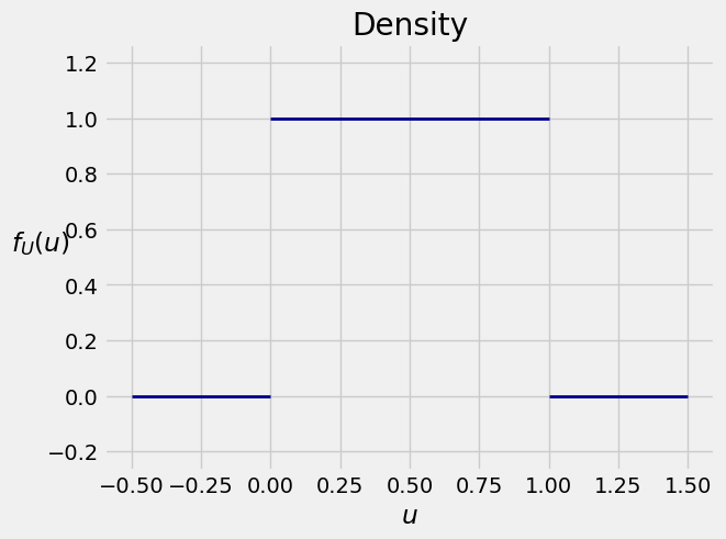
The area under
Equivalently, the cdf of
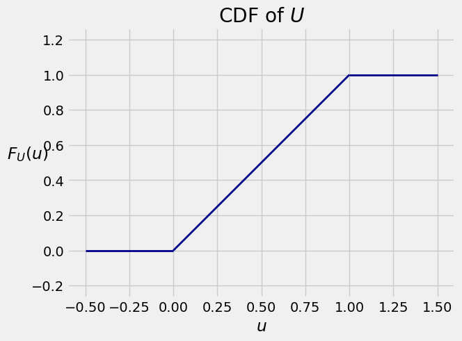
The expectation
For the variance, you do have to integrate. By the formula for expectation given at the start of this section,
15.3.2. Uniform
Fix
So if
and 0 elsewhere. Probabilities are still relative lengths, so the cdf of
The expectation and variance of
Step 1:
Step 2:
Step 3:
Now
which is the midpoint of
Quick Check
(a) Let
(b) Let
Answer
(a)
(b)
15.3.3. Example: Random Discs#
A screen saver chooses a random radius uniformly in the interval
Question 1. Let
Answer. Let
np.pi * (4/12 + 1)
4.1887902047863905
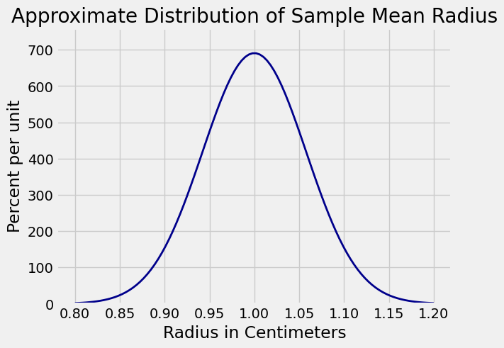
Question 2. Let
Answer. Let
sd_rbar = ((4/12)**0.5)/(100**0.5)
sd_rbar
0.057735026918962574
By the Central Limit Theorem, the distribution of Plot_norm.
Plot_norm((0.8, 1.2), 1, sd_rbar)
plt.xlabel('Radius in Centimeters')
plt.title('Approximate Distribution of Sample Mean Radius');
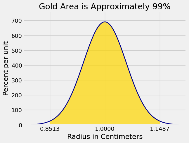
We are looking for
z = stats.norm.ppf(0.995)
z
2.5758293035489004
c = z*sd_rbar
c
0.14871557417904838
We can now get the endpoints of the interval. The graph below shows the corresponding area of 99%.
1-c, 1+c
(0.85128442582095165, 1.1487155741790485)
Plot_norm((0.8, 1.2), 1, sd_rbar, left_end = 1-c, right_end = 1+c)
plt.xticks([1-c, 1, 1+c])
plt.xlabel('Radius in Centimeters')
plt.title('Gold Area is Approximately 99%');
Quick Check
Let
Answer
Roughly normal, mean