16.2. Monotone Functions

If \(X\) is discrete, and \(g\) is a monotone function, then finding the distribution of the random variable \(Y = g(X)\) is straightforward: convert each possible value of \(X\) by applying \(g\) and leave the probabilities alone.

For example, if \(X\) is uniform on the three values \(0, 1, 2\), and \(Y = e^X\), then the you can just augment the distribution table of \(X\) by the possible values of \(Y\):

\(y\)	\(1\)	\(e\)	\(e^2\)
\(x\)	\(0\)	\(1\)	\(2\)
chance	\(\frac{1}{3}\)	\(\frac{1}{3}\)	\(\frac{1}{3}\)

The new random variable \(Y\) is uniform on the three values \(1, e, e^2\).

But if \(X\) has a density then both \(X\) and \(Y\) have a continuum of values and we have to be more careful.

The method we developed in the previous section for finding the density of a linear function of a random variable can be extended to non-linear functions.

See More

16.2.1. Change of Variable Formula for Density: Increasing Function

The function \(F^{-1}\) is differentiable and increasing. We will now develop a general method for finding the density of such a function applied to any random variable that has a density.

Let \(X\) have density \(f_X\). Let \(g\) be a smooth (that is, differentiable) increasing function, and let \(Y = g(X)\). Examples of such functions \(g\) are:

• \(g(x) = ax + b\) for some \(a > 0\). This case was covered in the previous section.

• \(g(x) = e^x\)

• \(g(x) = \sqrt{x}\) on positive values of \(x\)

To develop a formula for the density of \(Y\) in terms of \(f_X\) and \(g\), we will start with the cdf as we did above.

Let \(g\) be smooth and increasing, and let \(Y = g(X)\). We want a formula for \(f_Y\). We will start by finding a formula for the cdf \(F_Y\) of \(Y\) in terms of \(g\) and the cdf \(F_X\) of \(X\).

\[\begin{split} \begin{align*} F_Y(y) ~ & = ~ P(Y \le y) \\ &= ~ P(g(X) \le y) \\ &= ~ P(X \le g^{-1}(y)) ~~~~ \text{because } g \text{ is increasing} \\ &= ~ F_X(g^{-1}(y)) \end{align*} \end{split}\]

Now we can differentiate to find the density of \(Y\). By the chain rule and the fact that the derivative of an inverse is the reciprocal of the derivative,

\[\begin{split} \begin{align*} f_Y(y) ~ &= ~ f_X(g^{-1}(y)) \frac{d}{dy} g^{-1}(y) \\ &= ~ f_X(x) \frac{1}{g'(x)} ~~~~~ \text{at } x = g^{-1}(y) \end{align*} \end{split}\]

16.2.1.1. The Formula

Let \(g\) be a differentiable, increasing function. The density of \(Y = g(X)\) is given by

\[ f_Y(y) ~ = ~ \frac{f_X(x)}{g'(x)} ~~~ \text{at } x = g^{-1}(y) \]

16.2.2. Understanding the Formula

To see what is going on in the calculation, we will follow the same process as we used for linear functions in an earlier section.

• For \(Y\) to be \(y\), \(X\) has to be \(g^{-1}(y)\).

• Since \(g\) need not be linear, the tranformation by \(g\) won’t necessarily stretch the horizontal axis by a constant factor. Instead, the factor has different values at each \(x\). If \(g'\) denotes the derivative of \(g\), then the stretch factor at \(x\) is \(g'(x)\), the rate of change of \(g\) at \(x\). To make the total area under the density equal to 1, we have to compensate by dividing by \(g'(x)\). This is valid because \(g\) is increasing and hence \(g'\) is positive.

This gives us an intuitive justification for the formula.

16.2.3. Applying the Formula

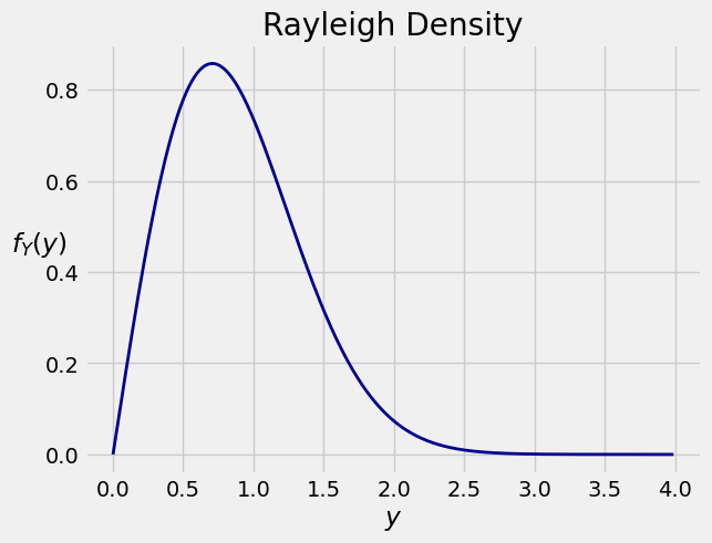
Let \(X\) have the exponential (1/2) density and let \(Y = \sqrt{X}\). We can take the square root because \(X\) is a positive random variable.

Let’s find the density of \(Y\) by applying the formula we have derived above. We will organize our calculation in four preliminary steps, and then plug into the formula.

• The density of the original random variable: The density of \(X\) is \(f_X(x) = (1/2)e^{-(1/2)x}\) for \(x > 0\).

• The function being applied to the original random variable: Take \(g(x) = \sqrt{x}\). Then \(g\) is increasing and its possible values are \((0, \infty)\).

• The inverse function: Let \(y = g(x) = \sqrt{x}\). We will now write \(x\) in terms of \(y\), to get \(x = y^2\).

• The derviative: The derivative of \(g\) is given by \(g'(x) = 1/(2\sqrt{x})\).

We are ready to plug this into our formula. Keep in mind that the possible values of \(Y\) are \((0, \infty)\). For \(y > 0\) the formula says

\[ f_Y(y) ~ = ~ \frac{f_X(x)} {g'(x)} ~~~ \text{at } x = g^{-1}(y) \]

So for \(y > 0\),

\[\begin{split} \begin{align*} f_Y(y) ~ &= ~ \frac{(1/2)e^{-\frac{1}{2}x}}{1/(2\sqrt{x})} ~~~~ \mbox{at } x = y^2 \\ &= ~ \sqrt{x} e^{-\frac{1}{2}x} ~~~~ \mbox{at } x = y^2 \\ &= ~ \sqrt{y^2} e^{-\frac{1}{2}y^2} \\ &= ~ y e^{-\frac{1}{2}y^2} \end{align*} \end{split}\]

This is called the Rayleigh density. Its graph is shown below.

Quick Check

\(V\) has density \(f_V(v) = 2v\) for \(v \in (0, 1)\) and 0 elsewhere. Let \(W = -\log(V)\). What are the possible values of \(W\)? What is the density of \(W\)?

Answer

Exponential \((2)\)

16.2.4. Change of Variable Formula for Density: Monotone Function

Let \(g\) be smooth and monotone (that is, either increasing or decreasing). The density of \(Y = g(X)\) is given by

\[ f_Y(y) ~ = ~ \frac{f_X(x)}{\lvert g'(x) \rvert} ~~~ \text{at } x = g^{-1}(y) \]

We have proved the result for increasing \(g\). When \(g\) is decreasing, the proof is analogous to proof in the linear case and accounts for \(g'\) being negative. We won’t take the time to write it out.

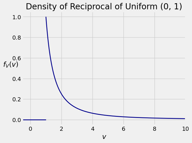
16.2.5. Reciprocal of a Uniform Variable

Let \(U\) be uniform on \((0, 1)\) and let \(V = 1/U\). The distribution of \(V\) is called the inverse uniform but the word “inverse” is confusing in the context of change of variable. So we will simply call \(V\) the reciprocal of \(U\).

To find the density of \(V\), start by noticing that the possible values of \(V\) are in \((1, \infty)\) as the possible values of \(U\) are in \((0, 1)\).

The components of the change of variable formula for densities:

• The original density: \(f_U(u) = 1\) for \(0 < u < 1\).

• The function: Define \(g(u) = 1/u\).

• The inverse function: Let \(v = g(u) = 1/u\). Then \(u = g^{-1}(v) = 1/v\).

• The derivative: Then \(g'(u) = -u^{-2}\).

By the formula, for \(v > 1\) we have

\[ f_V(v) ~ = ~ \frac{f_U(u)}{\lvert g'(u) \rvert} ~~~ \text{at } u = g^{-1}(v) \]

That is, for \(v > 1\),

\[ f_V(v) ~ = ~ 1 \cdot u^2 ~~~ \text{at } u = 1/v \]

So

\[ f_V(v) ~ = ~ \frac{1}{v^2}, ~~~ v > 1 \]

You should check that \(f_V\) is indeed a density, that is, it integrates to 1. You should also check that the expectation of \(V\) is infinite.

The density \(f_V\) belongs to the Pareto family of densities, much used in economics.