10.4.1. A Diffusion Model by Ehrenfest#

Paul Ehrenfest proposed a number of models for the diffusion of gas particles, one of which we will study here.

The model says that there are two containers containing a total of $N$ particles. At each instant, a container is selected at random and a particle is selected at random independently of the container. Then the selected particle is placed in the selected container; if it was already in that container, it stays there.

Let $X_n$ be the number of particles in Container 1 at time $n$. Then $X_0,X_1,\dots$ is a Markov chain with transition probabilities given by:

The chain is clearly irreducible. It is aperiodic because $P(i,i)>0$.

Question: What is the stationary distribution of the chain?

Answer: We have computers. So let’s first find the stationary distribution for $N=100$ particles, and then see if we can identify it for general $N$.

N = 100

states = np.arange(N+1)

def transition_probs(i, j):
    if j == i:
        return 1/2
    elif j == i+1:
        return (N-i)/(2*N)
    elif j == i-1:
        return i/(2*N)
    else:
        return 0

ehrenfest = MarkovChain.from_transition_function(states, transition_probs)
Plot(ehrenfest.steady_state(), edges=True)

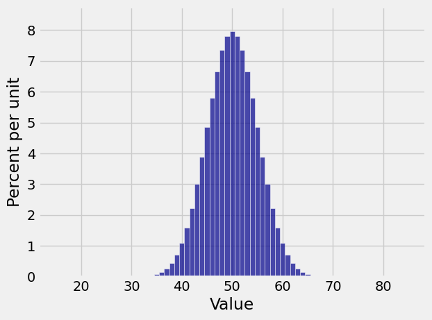
That looks suspiciously like the binomial (100, 1/2) distribution. In fact it is the binomial (100, 1/2) distribution. Let’s solve the balance equations to prove this.

The balance equations are:

Now rewrite each equation to express all the elements of $\pi$ in terms of $\pi (0)$. You will get:

and so on by induction:

This is true for $j=0$ as well, since $(\genfrac{}{}{0ex}{}{N}{0})=1$.

Therefore the stationary distribution is

In other words, the stationary distribution is proportional to the binomial coefficients. Now

So $\pi (0)=1/2^N$ and the stationary distribution is binomial $(N,1/2)$.

10.4.2. Expected Reward#

Suppose I run the sticky reflecting random walk from the previous section for a long time. As a reminder, here is its stationary distribution.

stationary = reflecting_walk.steady_state()
stationary

Question 1: Suppose that every time the chain is in state 4, I win 4 dollars; every time it’s in state 5, I win 5 dollars; otherwise I win nothing. What is my expected long run average reward?

Answer 1: In the long run, the chain is in steady state. So I expect that on 62.5% of the moves I will win nothing; on 25% of the moves I will win 4 dollars; and on 12.5% of the moves I will win 5 dollars. My expected long run average reward per move is 1.65 dollars.

0*0.625 + 4*0.25 + 5*.125

1.625

Question 2: Suppose that every time the chain is in state $i$, I toss $i$ coins and record the number of heads. In the long run, how many heads do I expect to get on average per move?

Answer 2: Each time the chain is in state $i$, I expect to get $i/2$ heads. When the chain is in steady state, the expected number of coins I toss at any given move is 3. So, by iterated expectations, the long run average number of heads I expect to get is 1.5.

stationary.ev()/2

1.5000000000000022

If that seems artificial, consider this: Suppose I play the game above, and on every move I tell you the number of heads that I get but I don’t tell you which state the chain is in. I hide the underlying Markov Chain. If you try to recreate the sequence of steps that the Markov Chain took, you are working with a Hidden Markov Model. These are much used in pattern recognition, bioinformatics, and other fields.