16.1.1. Linear Transformation: Exponential Density#

Let $T$ have the exponential $(\lambda )$ distribution and let $T_1=\lambda T$. Then $T_1$ is a linear transformation of $T$. Therefore

The parameter $\lambda$ has disappeared in these results. Let’s see how that follows from the distribution of $T_1$. The cdf of $T_1$ is

That’s the cdf of the exponential $(1)$ distribution, consistent with the expectation and SD we found above.

To summarize, if $T$ has the exponential $(\lambda )$ distribution then the distribution of $T_1=\lambda T$ is exponential $(1)$.

You can think of the exponential $(1)$ distribution as the fundamental member of the family of exponential distributions. All others in the family can be found by changing the scale of measurement, that is, by multiplying by a constant.

If $T_1$ has the exponential $(1)$ distribution, then $T=\frac{1}{\lambda }{T}_1$ has the exponential $(\lambda )$ distribution. The factor $1/\lambda$ is called the scale parameter.

Here are graphs of the densities of $T_1$ and $T=\frac{1}{2}{T}_1$. By the paragraph above, $T$ has the exponential $(2)$ distribution.

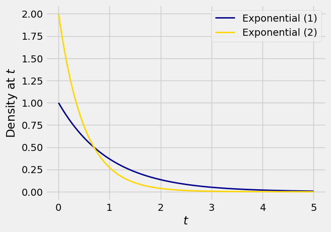
The formulas for the two densities are

Let’s try to understand the relation between these two densities in a way that will help us generalize what we are seeing in this example.

The relation between the two random variables is $T=\frac{1}{2}{T}_1$.

• For any $t$, the chance that $T$ is near $t$ is the same as the chance that $T_1$ is near $s=2t$. This explains the factor $e^{-2t}$ in the density of $T$.

• If we think of $T_1$ as a point on the horizontal axis, then to create $T$ you have to divide $T_1$ by $2$. So the transformation consists of halving all distances on the horizontal axis. The total area under the density of $T$ must equal $1$, so we have to compensate by doubling all distances on the vertical axis. This explains the factor $2$ in the density of $T$.

16.1.2. Linear Change of Variable Formula for Densities#

We use the same idea to find the density of a linear transformation of a random variable.

Let $X$ be a random variable with density $f_X$, and let $Y=aX+b$ for constants $a\ne 0$ and $b$. Let $f_Y$ be the density of $Y$. Then

Let’s take this formula in two pieces, as in the exponential example.

• For $Y$ to be $y$, $X$ has to be $(y-b)/a$.

• The linear function $y=ax+b$ involves multiplying distances along the horizontal axis by $|a|$; the sign of $a$ doesn’t affect distances. To get a density, we have to compensate by dividing all vertical distances by $|a|$.

This is a good way to understand the formula, and will help you understand the corresponding formula for non-linear transformations.

For a formal proof, start with the case $a>0$.

By the chain rule of differentiation,

If $a<0$ then division by $a$ causes the direction of the inequality to switch:

Now the chain rule yields

16.1.3. The Normal Densities#

Let $Z$ have the standard normal density

Let $X=\sigma Z+\mu$ for constants $\mu$ and $\sigma$ with $\sigma >0$. Then for any real number $x$, the density of $X$ is

Thus every normal random variable is a linear transformation of a standard normal variable.

16.1.4. The Uniform Densities, Revisited#

Let the distribution of $U$ be uniform on $(0,1)$ and for constants $b>a$ let $V=(b-a)U+a$. In an earlier section we saw that $V$ has the uniform distribution on $(a,b)$. But let’s see what’s involved in confirming that result using our new formula.

First it is a good idea to be clear about the possible values of $V$. Since the possible values of $U$ are in $(0,1)$, the possible values of $V$ are in $(a,b)$.

At $v\in (a,b)$, the density of $V$ is

That’s the uniform density on $(a,b)$.