Odds Ratios

6.5. Odds Ratios#

Binomial $(n, p)$ probabilities involve powers and factorials, both of which are difficult to compute when $n$ is large. This section is about simplifying the computation of the entire distribution. The result also helps us understand the shape of binomial histograms.

6.5.1. Consecutive Odds Ratios#

Fix $n$ and $p$ , and let $P (k)$ be the binomial $(n, p)$ probability of $k$ . That is, let $P (k)$ be the chance of getting $k$ successes in $n$ independent trials with probability $p$ of success on each trial.

The idea is to start at the left end of the distribution, with the term

P (0) = (1 - p)^{n}

Then we will build up the distribution recursively from left to right, one possible value at a time.

To do this, we have to know how the probabilities of consecutive values are related to each other. For $k \geq 1$ , define the $k$ th consecutive odds ratio

R (k) = \frac{P (k)}{P (k - 1)}

These ratios help us calculate $P (k)$ recursively.

\begin{array}{r} \begin{aligned} P (0) & = (1 - p)^{n} \\ P (1) & = P (0) \cdot \frac{P (1)}{P (0)} = P (0) R (1) \\ P (2) & = P (1) R (2) \end{aligned} \end{array}

and so on.

Even though we already have a formula for the binomial probabilities, building the distribution using consecutive ratios is better computationally and also helps us understand the shape of the distribution.

6.5.2. Binomial Consecutive Odds Ratios#

How is this more illuminating than plugging into the binomial formula? To see this, fix $k \geq 1$ and calculate the ratio $R (k)$ .

\begin{array}{r} \begin{aligned} R (k) & = \frac{(\binom{n}{k}) p^{k} (1 - p)^{n - k}}{(\binom{n}{k - 1}) p^{k - 1} (1 - p)^{n - k + 1}} \\ = \frac{n - k + 1}{k} \cdot \frac{p}{1 - p} (after cancellation) \end{aligned} \end{array}

Notice that the formulas for $R (k)$ are simple. This makes it easy to compute $P (k)$ recursively. For example, if $n \geq 3$ , we can compute $P (3)$ as

P (3) = (1 - p)^{n} (\frac{n - 1 + 1}{1} \cdot \frac{p}{1 - p}) (\frac{n - 2 + 1}{2} \cdot \frac{p}{1 - p}) (\frac{n - 3 + 1}{3} \cdot \frac{p}{1 - p})

Quick Check

In the binomial $(60, 2 / 3)$ distribution, $P (35) = 0.04207955004383654$ . Use this (but no scipy or combinatorics) to find $P (36)$ .

Answer

Multiply by $\frac{61 - 36}{36} \cdot 2$ to get $0.05844381950532852$ .

6.5.3. Shapes of Binomial Histograms#

Now observe that comparing $R (k)$ to 1 tells us whether the histogram is going up, staying level, or going down at $k$ .

\begin{array}{r} \begin{aligned} R (k) > 1 & ⟺ P (k) > P (k - 1) \\ R (k) = 1 & ⟺ P (k) = P (k - 1) \\ R (k) < 1 & ⟺ P (k) < P (k - 1) \end{aligned} \end{array}

Note also that the form

R (k) = (\frac{n + 1}{k} - 1) \cdot \frac{p}{1 - p}

tells us the the ratios are a decreasing function of $k$ . In the formula, $n$ and $p$ are the parameters of the distribution and hence constant. It is $k$ that varies, and $k$ appears in the denominator.

This implies that once $R (k) < 1$ for some $k$ , it will remain less than 1 for all larger $k$ . In other words, once the histogram starts going down, it will keep going down. It cannot come back up again.

That is why binomial histograms are either non-increasing or non-decreasing, or they go up and come down. But they can’t look like waves on the seashore. They can’t go up, come down, and go up again.

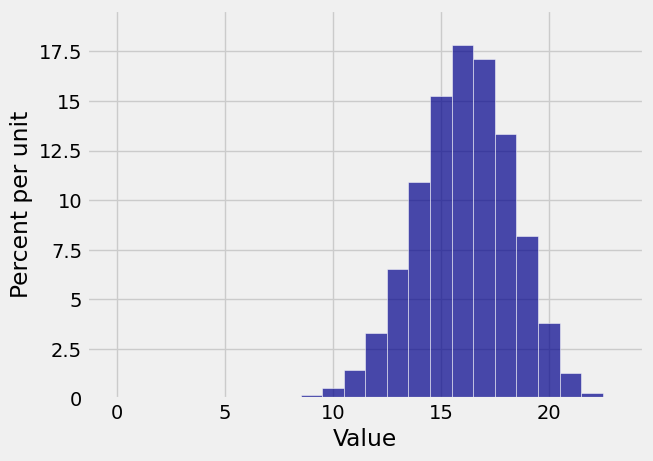
Let’s visualize this for a $n = 23$ and $p = 0.7$ , two parameters that have no significance other than being our choice to use in this example.

n = 23
p = 0.7
k = range(n+1)
bin_23_7 = stats.binom.pmf(k, n, p)
bin_dist = Table().values(k).probabilities(bin_23_7)
Plot(bin_dist)

../../_images/6b01f372cc03927f6129d88ce700ec99f04be3bdfba345cb9cda30ce77ce204a.png

# It is important to define k as an array here,
# so you can do array operations
# to find all the ratios at once.
k = np.arange(1, n+1, 1)
((n - k + 1)/k)*(p/(1-p))

array([ 53.66666667,  25.66666667,  16.33333333,  11.66666667,
         8.86666667,   7.        ,   5.66666667,   4.66666667,
         3.88888889,   3.26666667,   2.75757576,   2.33333333,
         1.97435897,   1.66666667,   1.4       ,   1.16666667,
         0.96078431,   0.77777778,   0.61403509,   0.46666667,
         0.33333333,   0.21212121,   0.10144928])

What Python is helpfully telling us is that the invisible bar at 1 is 53.666… times larger than the even more invisible bar at 0. The ratios decrease after that but they are still bigger than 1 through $k = 16$ . The histogram rises till it reaches its peak at $k = 16$ . You can see that $R (16) = 1.1666 > 1$ . Then the ratios drop below one, so the histogram starts going down.

6.5.4. Mode of the Binomial#

A mode of a discrete distribution is a possible value that has the highest probability. There may be more than one such value, so there may be more than one mode.

We have seen that once the ratio $R (k)$ drops below 1, it stays below 1, so the histogram keeps falling. To identify the mode, therefore, we will find all values of $k$ such that $R (k) \geq 1$ .

Let $q = 1 - p$ . Every value $k$ for which $R (k) \geq 1$ must satisfy

(\frac{n + 1}{k} - 1) \frac{p}{q} \geq 1

That is,

\frac{n + 1}{k} \geq \frac{q}{p} + 1 = \frac{1}{p}

which is equivalent to

k \leq (n + 1) p

We have shown that for all $k$ in the range 0 through the integer part of $(n + 1) p$ , the histogram rises; for larger $k$ , it falls.

Therefore the peak of the histogram is at the largest $k$ in this range. That’s the integer part of $(n + 1) p$ .

So the integer part of $(n + 1) p$ is a mode of the binomial.

Because the odds ratios are non-decreasing in $k$ , the only way in which there can be more than one mode is if there is a $k$ such that $R (k) = 1$ . In that case, $P (k) = P (k - 1)$ and therefore both $k$ and $k - 1$ will be modes. To summarize:

The mode of the binomial $(n, p)$ distribution is the integer part of $(n + 1) p$ . If $(n + 1) p$ is an integer, then $(n + 1) p - 1$ is also a mode.

To see that this is consistent with what we observed in our numerical example above, let’s calculate $(n + 1) p$ in that case.

(n+1) * p

16.799999999999997

The integer part of $(n + 1) p$ is 16, which is the mode that we observed.

But in fact, $n p$ is a more natural quantity to calculate. For example, if you are counting the number of heads in 100 tosses of a coin, then the distribution is binomial $(100, 1 / 2)$ and you naturally expect $n p = 50$ heads. You don’t want to be worrying about $101 \times (1 / 2)$ .

In fact you don’t have to worry when $n$ is large, because then $n p$ and $(n + 1) p$ are pretty close. In a later section we will examine a situation in which you can use $n p$ to get an approximation to the shape of the binomial distribution when $n$ is large.